2 Results
2.1 Overview
The following sections contain the main results reported in the paper.
The results are shown next to the R code that produced them.
Specifically, all code is written in RMarkdown which allows to combine analysis code with regular text.
The rendered RMarkdown files you see here, were generated automatically based on data stored in the relevant data sets listed above using continuous integration in the associated GitLab repository.
This means that upon any change to the analysis code, the relevant data is retrieved from the relevant sub-directories and all analyses are re-generated.
Please see the following sections for details on the computational environment and the continuous integration pipeline.
2.1.0.1 Computational environment
Below we show the version information about R, the operating system (OS) and attached or loaded R packages using sessionInfo()
## R version 4.0.3 (2020-10-10)
## Platform: x86_64-pc-linux-gnu (64-bit)
## Running under: Debian GNU/Linux bullseye/sid
##
## Matrix products: default
## BLAS: /usr/lib/x86_64-linux-gnu/openblas-pthread/libblas.so.3
## LAPACK: /usr/lib/x86_64-linux-gnu/openblas-pthread/libopenblasp-r0.3.10.so
##
## locale:
## [1] LC_CTYPE=en_US.UTF-8 LC_NUMERIC=C
## [3] LC_TIME=en_US.UTF-8 LC_COLLATE=en_US.UTF-8
## [5] LC_MONETARY=en_US.UTF-8 LC_MESSAGES=en_US.UTF-8
## [7] LC_PAPER=en_US.UTF-8 LC_NAME=C
## [9] LC_ADDRESS=C LC_TELEPHONE=C
## [11] LC_MEASUREMENT=en_US.UTF-8 LC_IDENTIFICATION=C
##
## attached base packages:
## [1] stats graphics grDevices utils datasets methods base
##
## loaded via a namespace (and not attached):
## [1] compiler_4.0.3 magrittr_1.5 bookdown_0.21 htmltools_0.5.0
## [5] tools_4.0.3 rstudioapi_0.11 yaml_2.2.1 stringi_1.5.3
## [9] rmarkdown_2.5 knitr_1.30 stringr_1.4.0 digest_0.6.27
## [13] xfun_0.18 rlang_0.4.8 evaluate_0.142.1.0.2 Continuous integration
Below we show the continuous integration script that was used to automatically generate this project website. This is made possible by using thee great tools DataLad and bookdown.
stages:
- retrieve
- publish
datalad:
stage: retrieve
image:
name: registry.git.mpib-berlin.mpg.de/wittkuhn/highspeed/datalad:0.13.5
entrypoint: [""]
script:
# rclone configurations:
- rclone config create highspeed-bids seafile url https://keeper.mpdl.mpg.de/ user wittkuhn@mpib-berlin.mpg.de library highspeed-bids pass $CI_KEEPER_PASS
- rclone config create highspeed-analysis seafile url https://keeper.mpdl.mpg.de/ user wittkuhn@mpib-berlin.mpg.de library highspeed-analysis pass $CI_KEEPER_PASS
#- rclone config create highspeed-fmriprep seafile url https://keeper.mpdl.mpg.de/ user wittkuhn@mpib-berlin.mpg.de library highspeed-fmriprep pass $CI_KEEPER_PASS
- rclone config create highspeed-mriqc seafile url https://keeper.mpdl.mpg.de/ user wittkuhn@mpib-berlin.mpg.de library highspeed-mriqc pass $CI_KEEPER_PASS
- rclone config create highspeed-masks seafile url https://keeper.mpdl.mpg.de/ user wittkuhn@mpib-berlin.mpg.de library highspeed-masks pass $CI_KEEPER_PASS
- rclone config create highspeed-glm seafile url https://keeper.mpdl.mpg.de/ user wittkuhn@mpib-berlin.mpg.de library highspeed-glm pass $CI_KEEPER_PASS
# git configuration:
- git config --global user.name "GitLab CI"
- git config --global user.email "ci@git.mpib-berlin.mpg.de"
# remove and install all datasets:
- datalad remove --dataset . bibliography
- datalad clone --dataset . https://github.com/lnnrtwttkhn/bibliography.git
#- datalad remove --dataset . highspeed-analysis
- rm -rf highspeed-analysis
- datalad install --dataset . -r https://github.com/lnnrtwttkhn/highspeed-analysis.git
- datalad remove --dataset . highspeed-bids
- datalad clone --dataset . https://github.com/lnnrtwttkhn/highspeed-bids.git
- datalad remove --dataset . highspeed-fmriprep
- datalad clone --dataset . https://github.com/lnnrtwttkhn/highspeed-fmriprep.git
- datalad remove --dataset . highspeed-mriqc
- datalad clone --dataset . https://github.com/lnnrtwttkhn/highspeed-mriqc.git
- datalad remove --dataset . highspeed-masks
- datalad clone --dataset . https://github.com/lnnrtwttkhn/highspeed-masks.git
- datalad remove --dataset . highspeed-glm
- datalad clone --dataset . https://github.com/lnnrtwttkhn/highspeed-glm.git
- datalad remove --dataset . highspeed-decoding
- datalad clone --dataset . https://github.com/lnnrtwttkhn/highspeed-decoding.git
# add gin siblings for all datasets:
- datalad siblings add --dataset highspeed-bids -s gin --url https://gin.g-node.org/lnnrtwttkhn/highspeed-bids
- datalad siblings add --dataset highspeed-analysis -s gin --url https://gin.g-node.org/lnnrtwttkhn/highspeed-analysis
- datalad siblings add --dataset highspeed-analysis/data/bids -s gin --url https://gin.g-node.org/lnnrtwttkhn/highspeed-bids
- datalad siblings add --dataset highspeed-analysis/data/decoding -s gin --url https://gin.g-node.org/lnnrtwttkhn/highspeed-decoding
#- datalad siblings add --dataset highspeed-fmriprep -s gin --url https://gin.g-node.org/lnnrtwttkhn/highspeed-fmriprep
- datalad siblings add --dataset highspeed-mriqc -s gin --url https://gin.g-node.org/lnnrtwttkhn/highspeed-mriqc
- datalad siblings add --dataset highspeed-masks -s gin --url https://gin.g-node.org/lnnrtwttkhn/highspeed-masks
- datalad siblings add --dataset highspeed-glm -s gin --url https://gin.g-node.org/lnnrtwttkhn/highspeed-glm
- datalad siblings add --dataset highspeed-decoding -s gin --url https://gin.g-node.org/lnnrtwttkhn/highspeed-decoding
# enable keeper siblings for all datasets:
- datalad siblings --dataset highspeed-analysis enable --name keeper
- datalad siblings --dataset highspeed-bids enable --name keeper
- datalad siblings --dataset highspeed-analysis/data/bids enable --name keeper
#- datalad siblings --dataset highspeed-fmriprep enable --name keeper
- datalad siblings --dataset highspeed-mriqc enable --name keeper
- datalad siblings --dataset highspeed-masks enable --name keeper
- datalad siblings --dataset highspeed-glm enable --name keeper
# configure gin and keeper siblings for all datasets:
- datalad siblings --dataset highspeed-bids configure --name origin --publish-depends gin --publish-depends keeper
- datalad siblings --dataset highspeed-analysis configure --name origin --publish-depends gin
- datalad siblings --dataset highspeed-analysis/data/bids configure --name origin --publish-depends gin --publish-depends keeper
#- datalad siblings --dataset highspeed-fmriprep configure --name origin --publish-depends gin --publish-depends keeper
- datalad siblings --dataset highspeed-mriqc configure --name origin --publish-depends gin --publish-depends keeper
- datalad siblings --dataset highspeed-masks configure --name origin --publish-depends gin --publish-depends keeper
- datalad siblings --dataset highspeed-glm configure --name origin --publish-depends gin --publish-depends keeper
- datalad siblings --dataset highspeed-decoding configure --name origin --publish-depends gin
- datalad siblings --dataset highspeed-analysis/data/decoding configure --name origin --publish-depends gin
# get data
- datalad get highspeed-analysis/data/bids/participants.tsv
- datalad get highspeed-analysis/data/bids/sub-*/ses-*/func/*events.tsv || true
- datalad get highspeed-analysis/data/bids/sub-*/ses-*/func/*events.tsv
- datalad get highspeed-analysis/data/decoding/decoding/sub-*/data/*_decoding.csv || true
- datalad get highspeed-analysis/data/decoding/decoding/sub-*/data/*_decoding.csv
- datalad get highspeed-analysis/data/decoding/decoding/*/data/*thresholding.csv || true
- datalad get highspeed-analysis/data/decoding/decoding/*/data/*thresholding.csv
- datalad get highspeed-analysis/data/tmp/dt_pred_conc_slope.Rdata
artifacts:
paths:
- bibliography/code/bibliography.bib
- highspeed-bids/code
- highspeed-analysis/code
- highspeed-analysis/figures
- highspeed-analysis/sourcedata
- highspeed-analysis/data/bids/sub-*/ses-*/func/*events.tsv
- highspeed-analysis/data/decoding/decoding/sub-*/data/*_decoding.csv
- highspeed-analysis/data/decoding/decoding/sub-*/data/*_thresholding.csv
- highspeed-analysis/data/tmp
- highspeed-fmriprep/code
- highspeed-mriqc/code
- highspeed-glm/code
- highspeed-decoding/code
expire_in: 1 hour
only:
- master
pages:
stage: publish
image: registry.git.mpib-berlin.mpg.de/wittkuhn/highspeed/bookdown:latest
script:
- Rscript -e "options(bookdown.render.file_scope = FALSE); bookdown::render_book('index.Rmd', 'all', output_dir = 'public')"
artifacts:
paths:
- public
- highspeed-analysis/figures
- highspeed-analysis/sourcedata
only:
- master2.2 Behavior
2.2.1 Initialization
2.2.1.1 Load data and files
We set the paths and source the basic setup script:
knitr::opts_chunk$set(echo = TRUE)
# find the path to the root of this project:
if (!requireNamespace("here")) install.packages("here")
if ( basename(here::here()) == "highspeed" ) {
path_root = here::here("highspeed-analysis")
} else {
path_root = here::here()
}
# source all relevant functions from the setup R script:
source(file.path(path_root, "code", "highspeed-analysis-setup.R"))2.2.1.2 Signal-detection labeling
We assign labels from signal detection theory that will be used in one of the analyses below:
# denotes misses (key was not pressed and stimulus was upside-down):
dt_events$sdt_type[
dt_events$key_down == 0 & dt_events$stim_orient == 180] <- "miss"
# denotes hits (key was pressed and stimulus was upside-down):
dt_events$sdt_type[
dt_events$key_down == 1 & dt_events$stim_orient == 180] <- "hit"
# denotes correct rejection (key was not pressed and stimulus was upright):
dt_events$sdt_type[
dt_events$key_down == 0 & dt_events$stim_orient == 0] <- "correct rejection"
# denotes false alarms (key was pressed and stimulus was upright):
dt_events$sdt_type[
dt_events$key_down == 1 & dt_events$stim_orient == 0] <- "false alarm"2.2.2 Stimulus timings
We calculate the differences between consecutive stimulus onsets:
dt_events %>%
# get duration of stimuli by calculating differences between consecutive onsets:
.[, duration_check := shift(onset, type = "lead") - onset,
by = .(subject, run_study)] %>%
# get the difference between the expected and actual stimulus duration:
.[, duration_diff := duration_check - duration, by = .(subject, run_study)] %>%
# for each condition and trial check participants' responses:
.[, by = .(subject, condition, trial), ":=" (
# for each trial check if a key has been pressed:
trial_key_down = ifelse(any(key_down == 1, na.rm = TRUE), 1, 0),
# for each trial check if the participant was accurate:
trial_accuracy = ifelse(any(accuracy == 1, na.rm = TRUE), 1, 0)
)] %>%
.[, trial_type := factor(trial_type, levels = rev(unique(trial_type)))]timings_summary = dt_events %>%
filter(condition %in% c("sequence", "repetition") & trial_type == "interval") %>%
setDT(.) %>%
.[, by = .(subject, condition, trial_type), {
results = t.test(duration_diff, mu = 0.001, alternative = "two.sided")
list(
mean = mean(duration_diff, na.rm = TRUE),
sd = sd(duration_diff, na.rm = TRUE),
min = min(duration_diff, na.rm = TRUE),
max = max(duration_diff, na.rm = TRUE),
num = .N,
tvalue = results$statistic,
df = results$parameter,
pvalue = results$p.value,
pvalue_round = round_pvalues(results$p.value)
)
}] %>%
.[, trial_type := factor(trial_type, levels = rev(unique(trial_type)))] %>%
setorder(., condition, trial_type)
rmarkdown::paged_table(timings_summary)We plot the differences in expected versus actual timings of individual stimuli in the behavioral task:
ggplot(data = dt_events, aes(
y = as.numeric(duration_diff),
x = as.factor(trial_type),
fill = as.factor(trial_type)), na.rm = TRUE) +
facet_grid(vars(as.factor(trial_key_down)), vars(as.factor(condition))) +
geom_point(
aes(y = as.numeric(duration_diff), color = as.factor(trial_type)),
position = position_jitter(width = .15), size = .5, alpha = 1, na.rm = TRUE) +
geom_boxplot(width = .1, outlier.shape = NA, alpha = 0.5, na.rm = TRUE) +
scale_color_brewer(palette = "Spectral") +
scale_fill_brewer(palette = "Spectral") +
#coord_capped_flip(left = "both", bottom = "both", expand = TRUE) +
coord_flip() +
theme(legend.position = "none") +
xlab("Trial event (in serial order)") +
ylab("Difference between expected and actual timing (in s)") +
theme(strip.text = element_text(margin = margin(unit(c(t = 2, r = 2, b = 2, l = 2), "pt")))) +
theme(legend.position = "none") +
theme(panel.background = element_blank())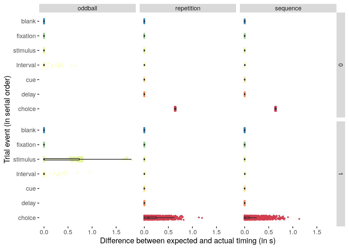
We check the timing of the inter-trial interval on oddball trials:
dt_odd_iti_mean = dt_events %>%
# filter for the stimulus intervals on oddball trials:
filter(condition == "oddball" & trial_type == "interval") %>%
setDT(.) %>%
# calculate the mean duration of the oddball intervals for each participant:
.[, by = .(subject), .(
mean_duration = mean(duration, na.rm = TRUE),
num_trials = .N
)] %>%
verify(num_trials == 600)
rmarkdown::paged_table(head(dt_odd_iti_mean))2.2.3 Behavioral performance
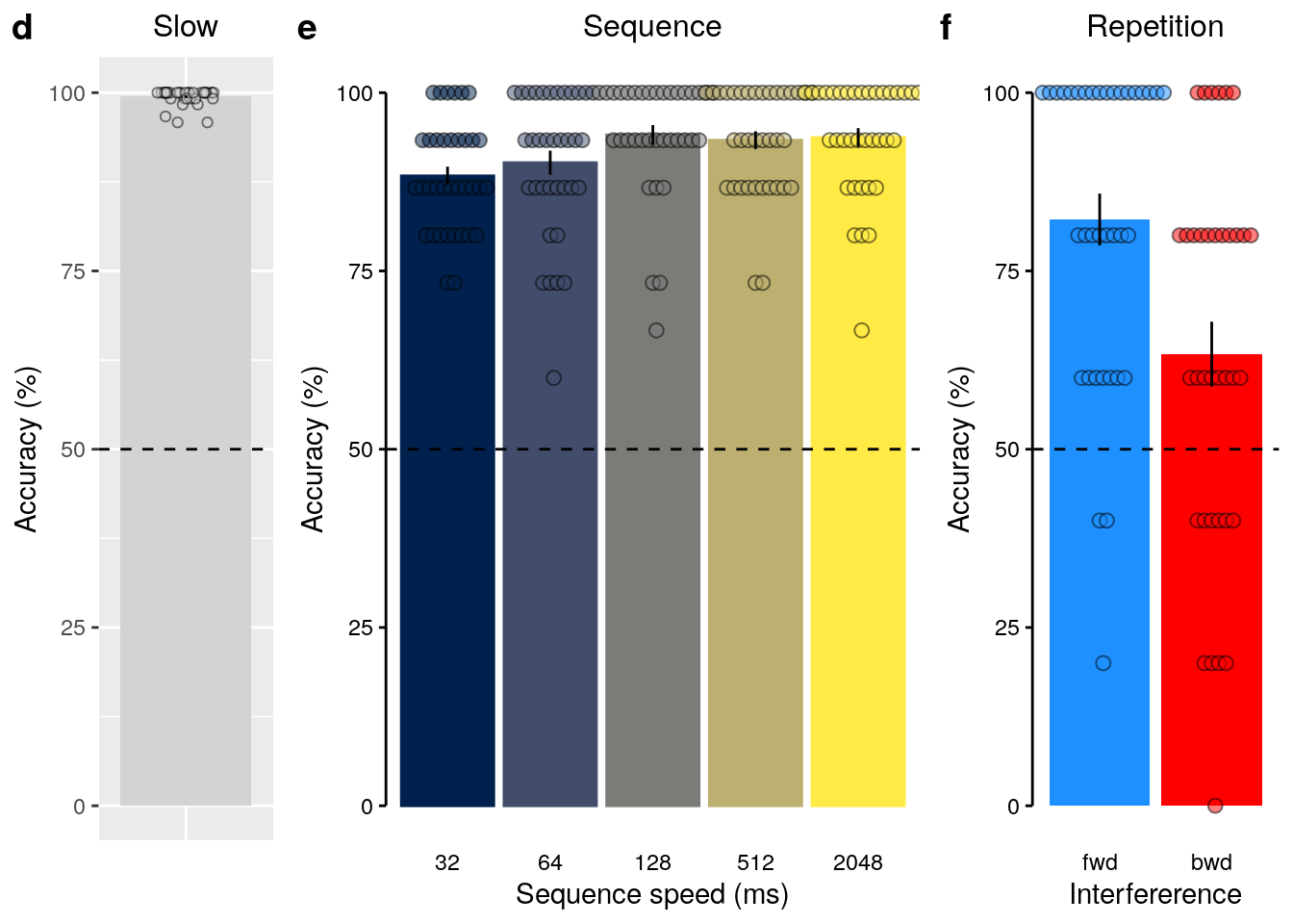
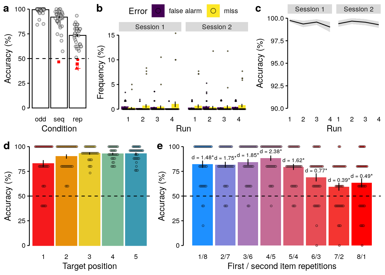
2.2.3.1 Mean accuracy
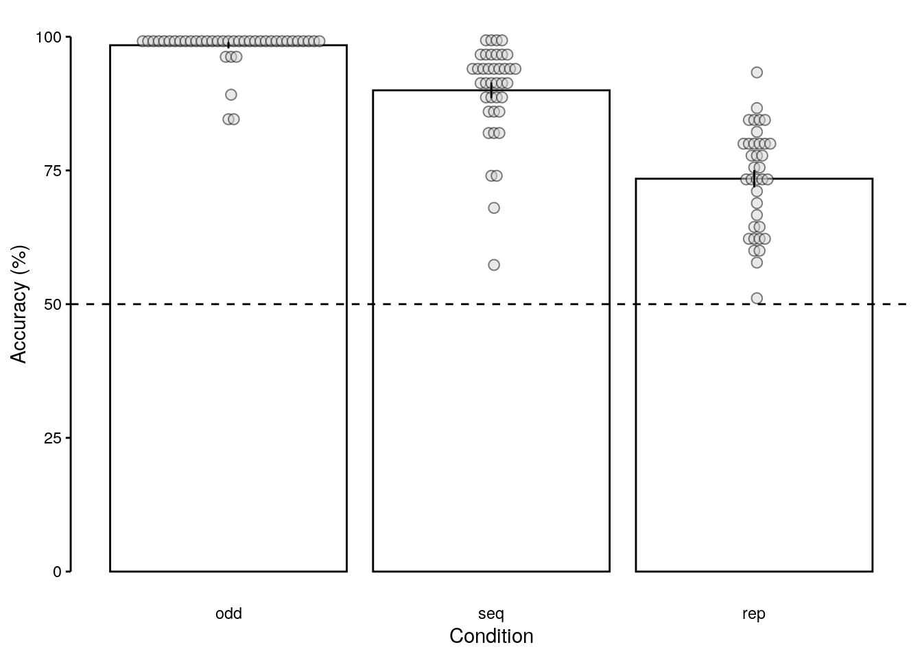
We calculate the mean behavioral accuracy across all trials of all three task conditions (slow, sequence, and repetition trials):
# behavioral chance level is at 50%:
chance_level = 50
dt_acc = dt_events %>%
# filter out all events that are not related to a participants' response:
filter(!is.nan(accuracy)) %>%
# filter for only upside down stimuli on slow trials:
filter(!(condition == "oddball" & stim_orient == 0)) %>%
setDT(.) %>%
# check if the number of trials matches for every subject:
verify(.[(condition == "oddball"), by = .(subject), .(
num_trials = .N)]$num_trials == 120) %>%
verify(.[(condition == "sequence"), by = .(subject), .(
num_trials = .N)]$num_trials == 75) %>%
verify(.[(condition == "repetition"), by = .(subject), .(
num_trials = .N)]$num_trials == 45) %>%
# calculate the average accuracy for each participant and condition:
.[, by = .(subject, condition), .(
mean_accuracy = mean(accuracy, na.rm = TRUE) * 100,
num_trials = .N)] %>%
# check if the accuracy values are between 0 and 100:
assert(within_bounds(lower.bound = 0, upper.bound = 100), mean_accuracy) %>%
# create new variable that specifies excluded participants:
mutate(exclude = ifelse(mean_accuracy < chance_level, "yes", "no")) %>%
# create a short name for the conditions:
mutate(condition_short = substr(condition, start = 1, stop = 3)) %>%
# reorder the condition factor in descending order of accuracy:
transform(condition_short = fct_reorder(
condition_short, mean_accuracy, .desc = TRUE))
rmarkdown::paged_table(dt_acc)We create a list of participants that will be excluded because their performance is below the 50% chance level in either or both sequence and repetition trials:
# create a list with all excluded subject ids and print the list:
subjects_excluded = unique(dt_acc$subject[dt_acc$exclude == "yes"])
print(subjects_excluded)## [1] "sub-24" "sub-31" "sub-37" "sub-40"We calculate the mean behavioral accuracy across all three task conditions (slow, sequence, and repetition trials), excluding participants that performed below chance on either or both sequence and repetition trials:
dt_acc_mean = dt_acc %>%
# filter out all data of excluded participants:
filter(!(subject %in% unique(subject[exclude == "yes"]))) %>%
# check if the number of participants matches expectations:
verify(length(unique(subject)) == 36) %>%
setDT(.) %>%
# calculate mean behavioral accuracy across participants for each condition:
.[, by = .(condition), {
ttest_results = t.test(
mean_accuracy, mu = chance_level, alternative = "greater")
list(
pvalue = ttest_results$p.value,
pvalue_rounded = round_pvalues(ttest_results$p.value),
tvalue = round(ttest_results$statistic, digits = 2),
conf_lb = round(ttest_results$conf.int[1], digits = 2),
conf_ub = round(ttest_results$conf.int[2], digits = 2),
df = ttest_results$parameter,
num_subs = .N,
mean_accuracy = round(mean(mean_accuracy), digits = 2),
SD = round(sd(mean_accuracy), digits = 2),
cohens_d = round((mean(mean_accuracy) - chance_level) / sd(mean_accuracy), 2),
sem_upper = mean(mean_accuracy) + (sd(mean_accuracy)/sqrt(.N)),
sem_lower = mean(mean_accuracy) - (sd(mean_accuracy)/sqrt(.N))
)}] %>%
verify(num_subs == 36) %>%
# create a short name for the conditions:
mutate(condition_short = substr(condition, start = 1, stop = 3)) %>%
# reorder the condition factor in descending order of accuracy:
transform(condition_short = fct_reorder(condition_short, mean_accuracy, .desc = TRUE))
# show the table (https://rstudio.github.io/distill/tables.html):
rmarkdown::paged_table(dt_acc_mean)2.2.3.2 Above-chance performance
We plot only data of above-chance performers:
2.2.3.3 Figure S1a
We plot data of all participants with below chance performers highlighted in red.
fig_behav_all_outlier = ggplot(data = dt_acc_mean,
mapping = aes(x = as.factor(condition_short), y = as.numeric(mean_accuracy),
group = as.factor(condition_short), fill = as.factor(condition_short))) +
geom_bar(aes(fill = as.factor(condition)), stat = "identity",
color = "black", fill = "white") +
geom_point(data = subset(dt_acc, exclude == "no"),
aes(color = as.factor(exclude)),
position = position_jitter(width = 0.2, height = 0, seed = 2),
alpha = 0.5, inherit.aes = TRUE, pch = 21,
color = "black", fill = "lightgray") +
geom_point(data = subset(dt_acc, exclude == "yes"),
aes(color = as.factor(exclude), shape = as.factor(subject)),
position = position_jitter(width = 0.05, height = 0, seed = 4),
alpha = 1, inherit.aes = TRUE, color = "red") +
geom_errorbar(aes(ymin = sem_lower, ymax = sem_upper), width = 0.0, color = "black") +
ylab("Accuracy (%)") + xlab("Condition") +
scale_color_manual(values = c("darkgray", "red"), name = "Outlier") +
geom_hline(aes(yintercept = 50), linetype = "dashed", color = "black") +
coord_capped_cart(left = "both", bottom = "none", expand = TRUE, ylim = c(0, 100)) +
theme(axis.ticks.x = element_line(color = "white"),
axis.line.x = element_line(color = "white")) +
guides(shape = FALSE, fill = FALSE) +
theme(axis.text = element_text(color = "black")) +
theme(axis.ticks = element_line(color = "black")) +
theme(axis.line.y = element_line(colour = "black"),
axis.ticks.x = element_blank(),
panel.grid.major = element_blank(),
panel.grid.minor = element_blank(),
panel.border = element_blank(),
panel.background = element_blank())
fig_behav_all_outlier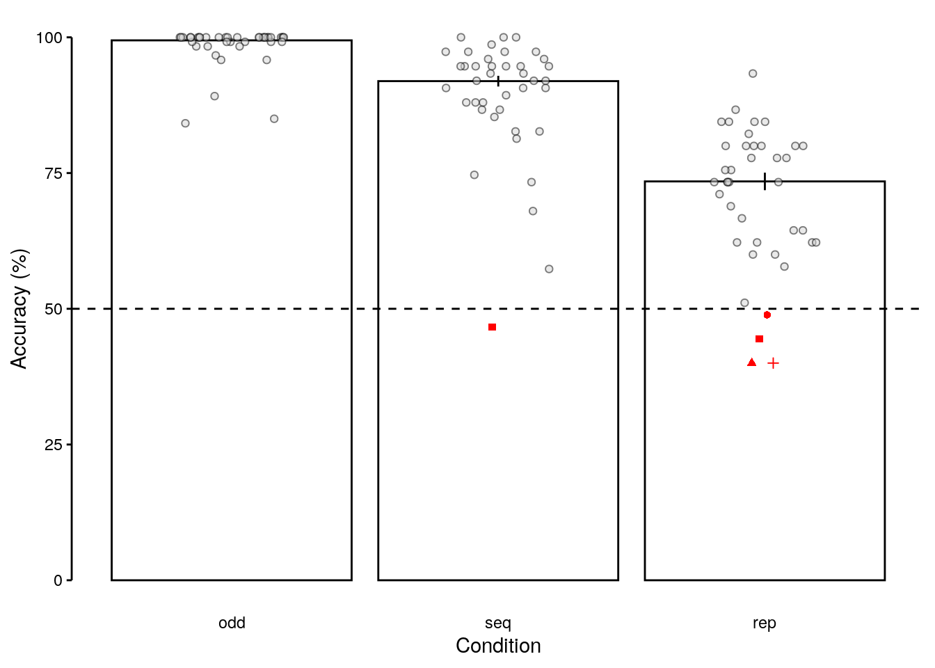
2.2.3.4 Source Data File Fig. S1a
dt_acc %>%
select(-num_trials) %>%
write.csv(., file = file.path(path_sourcedata, "source_data_figure_s1a.csv"),
row.names = FALSE)2.2.4 Slow trials
2.2.4.1 Mean accuracy (all trials)
We calculate the mean accuracy on slow trials (oddball task condition) across all trials in the final sample (only participants who performed above chance):
# we use the dataframe containing the accuracy data
dt_acc_odd = dt_acc %>%
# filter for oddball / slow trials only:
filter(condition == "oddball") %>%
# exclude participants with below chance performance::
filter(!(subject %in% subjects_excluded)) %>%
# verify that the number of participants (final sample) is correct:
verify(all(.N == 36))We plot the mean behavioral accuracy on slow trials (oddball task condition) in the final sample:
fig_behav_odd = ggplot(data = dt_acc_odd, aes(
x = "mean_acc", y = as.numeric(mean_accuracy))) +
geom_bar(stat = "summary", fun = "mean", fill = "lightgray") +
#geom_dotplot(binaxis = "y", stackdir = "center", stackratio = 0.5,
# color = "black", fill = "lightgray", alpha = 0.5,
# inherit.aes = TRUE, binwidth = 0.5) +
geom_point(position = position_jitter(width = 0.2, height = 0, seed = 2),
alpha = 0.5, inherit.aes = TRUE, pch = 21,
color = "black", fill = "lightgray") +
geom_errorbar(stat = "summary", fun.data = "mean_se", width = 0.0, color = "black") +
ylab("Accuracy (%)") + xlab("Condition") +
scale_color_manual(values = c("darkgray", "red"), name = "Outlier") +
geom_hline(aes(yintercept = 50), linetype = "dashed", color = "black") +
#coord_capped_cart(left = "both", bottom = "none", expand = TRUE, ylim = c(90, 100)) +
theme(plot.title = element_text(size = 12, face = "plain")) +
theme(axis.ticks.x = element_line(color = "white"),
axis.line.x = element_line(color = "white")) +
theme(axis.title.x = element_text(color = "white"),
axis.text.x = element_text(color = "white")) +
ggtitle("Slow") +
theme(plot.title = element_text(hjust = 0.5))
fig_behav_odd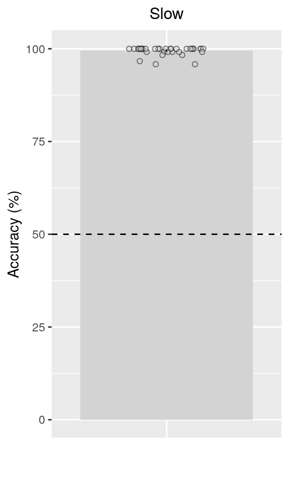
2.2.4.2 Mean accuracy (per run)
We calculate the mean behavioral accuracy on slow trials (oddball task condition) for each of the eight task runs for each participant:
# calculate the mean accuracy per session and run for every participant:
dt_odd_behav_run_sub = dt_events %>%
# exclude participants performing below chance:
filter(!(subject %in% subjects_excluded)) %>%
# select only oddball condition and stimulus events:
filter(condition == "oddball" & trial_type == "stimulus") %>%
# filter for upside-down trials (oddballs) only:
filter(stim_orient == 180) %>%
setDT(.) %>%
# calculate mean accuracy per session and run:
.[, by = .(subject, session, run_study, run_session), .(
mean_accuracy = mean(accuracy))] %>%
# express accuracy in percent by multiplying with 100:
transform(mean_accuracy = mean_accuracy * 100) %>%
# check whether the mean accuracy is within the expected range of 0 to 100:
assert(within_bounds(lower.bound = 0, upper.bound = 100), mean_accuracy)We calculate the mean behavioral accuracy on slow trials (oddball task condition) for each of the eight task runs across participants:
# calculate mean accuracy per session and run across participants:
dt_odd_behav_run_mean = dt_odd_behav_run_sub %>%
setDT(.) %>%
# average across participants:
.[, by = .(session, run_study, run_session), .(
mean_accuracy = mean(mean_accuracy),
num_subs = .N,
sem_upper = mean(mean_accuracy) + (sd(mean_accuracy)/sqrt(.N)),
sem_lower = mean(mean_accuracy) - (sd(mean_accuracy)/sqrt(.N))
)] %>%
verify(num_subs == 36) %>%
# z-score the accuracy values:
mutate(mean_accuracy_z = scale(mean_accuracy, scale = TRUE, center = TRUE))We run a LME model to test the linear effect of task run on behavioral accuracy:
lme_odd_behav_run = lmerTest::lmer(
mean_accuracy ~ run_study + (1 + run_study | subject),
data = dt_odd_behav_run_sub, na.action = na.omit, control = lcctrl)
summary(lme_odd_behav_run)
anova(lme_odd_behav_run)## Linear mixed model fit by REML. t-tests use Satterthwaite's method [
## lmerModLmerTest]
## Formula: mean_accuracy ~ run_study + (1 + run_study | subject)
## Data: dt_odd_behav_run_sub
## Control: lcctrl
##
## REML criterion at convergence: 1250.2
##
## Scaled residuals:
## Min 1Q Median 3Q Max
## -6.7158 0.1095 0.1285 0.1571 1.9026
##
## Random effects:
## Groups Name Variance Std.Dev. Corr
## subject (Intercept) 0.12000 0.3464
## run_study 0.01038 0.1019 1.00
## Residual 3.97535 1.9938
## Number of obs: 288, groups: subject, 36
##
## Fixed effects:
## Estimate Std. Error df t value Pr(>|t|)
## (Intercept) 99.53650 0.26529 135.52431 375.201 <2e-16 ***
## run_study -0.01969 0.05401 92.71468 -0.365 0.716
## ---
## Signif. codes: 0 '***' 0.001 '**' 0.01 '*' 0.05 '.' 0.1 ' ' 1
##
## Correlation of Fixed Effects:
## (Intr)
## run_study -0.757
## Type III Analysis of Variance Table with Satterthwaite's method
## Sum Sq Mean Sq NumDF DenDF F value Pr(>F)
## run_study 0.52843 0.52843 1 92.715 0.1329 0.7162We run a second model to test run- and session-specific effects:
dt <- dt_odd_behav_run_sub %>%
transform(run_session = as.factor(paste0("run-0", run_session)),
session = as.factor(paste0("ses-0", session)))lme_odd_behav_run = lmerTest::lmer(
mean_accuracy ~ session + run_session + (1 + session + run_session | subject),
data = dt, na.action = na.omit, control = lcctrl)
summary(lme_odd_behav_run)
emmeans(lme_odd_behav_run, list(pairwise ~ run_session | session))
anova(lme_odd_behav_run)
rm(dt)## Linear mixed model fit by REML. t-tests use Satterthwaite's method [
## lmerModLmerTest]
## Formula: mean_accuracy ~ session + run_session + (1 + session + run_session |
## subject)
## Data: dt
## Control: lcctrl
##
## REML criterion at convergence: 1192.3
##
## Scaled residuals:
## Min 1Q Median 3Q Max
## -4.2095 -0.0252 0.1378 0.2041 2.8277
##
## Random effects:
## Groups Name Variance Std.Dev. Corr
## subject (Intercept) 0.1958 0.4425
## sessionses-02 2.2398 1.4966 -0.73
## run_sessionrun-02 0.4736 0.6882 0.44 0.09
## run_sessionrun-03 0.8393 0.9161 0.70 -0.01 0.78
## run_sessionrun-04 4.2997 2.0736 0.90 -0.77 0.02 0.47
## Residual 2.4305 1.5590
## Number of obs: 288, groups: subject, 36
##
## Fixed effects:
## Estimate Std. Error df t value Pr(>|t|)
## (Intercept) 99.544925 0.218252 85.583815 456.101 <2e-16 ***
## sessionses-02 0.049649 0.309796 35.649869 0.160 0.874
## run_sessionrun-02 -0.054933 0.284024 67.397962 -0.193 0.847
## run_sessionrun-03 -0.009178 0.301376 54.333815 -0.030 0.976
## run_sessionrun-04 -0.423351 0.432376 37.096544 -0.979 0.334
## ---
## Signif. codes: 0 '***' 0.001 '**' 0.01 '*' 0.05 '.' 0.1 ' ' 1
##
## Correlation of Fixed Effects:
## (Intr) sss-02 rn_-02 rn_-03
## sessinss-02 -0.447
## rn_sssnr-02 -0.485 0.031
## rn_sssnr-03 -0.394 -0.006 0.555
## rn_sssnr-04 -0.115 -0.498 0.281 0.449
## $`emmeans of run_session | session`
## session = ses-01:
## run_session emmean SE df lower.CL upper.CL
## run-01 99.54 0.2183 35 99.10 99.99
## run-02 99.49 0.2611 35 98.96 100.02
## run-03 99.54 0.2943 35 98.94 100.13
## run-04 99.12 0.4614 35 98.18 100.06
##
## session = ses-02:
## run_session emmean SE df lower.CL upper.CL
## run-01 99.59 0.2883 35 99.01 100.18
## run-02 99.54 0.3302 35 98.87 100.21
## run-03 99.59 0.3478 35 98.88 100.29
## run-04 99.17 0.3389 35 98.48 99.86
##
## Degrees-of-freedom method: kenward-roger
## Confidence level used: 0.95
##
## $`pairwise differences of run_session | session`
## session = ses-01:
## contrast estimate SE df t.ratio p.value
## (run-01) - (run-02) 0.05493 0.284 35 0.193 0.9974
## (run-01) - (run-03) 0.00918 0.301 35 0.030 1.0000
## (run-01) - (run-04) 0.42335 0.432 35 0.979 0.7621
## (run-02) - (run-03) -0.04575 0.277 35 -0.165 0.9984
## (run-02) - (run-04) 0.36842 0.446 35 0.827 0.8415
## (run-03) - (run-04) 0.41417 0.401 35 1.033 0.7314
##
## session = ses-02:
## contrast estimate SE df t.ratio p.value
## (run-01) - (run-02) 0.05493 0.284 35 0.193 0.9974
## (run-01) - (run-03) 0.00918 0.301 35 0.030 1.0000
## (run-01) - (run-04) 0.42335 0.432 35 0.979 0.7621
## (run-02) - (run-03) -0.04575 0.277 35 -0.165 0.9984
## (run-02) - (run-04) 0.36842 0.446 35 0.827 0.8415
## (run-03) - (run-04) 0.41417 0.401 35 1.033 0.7314
##
## Degrees-of-freedom method: kenward-roger
## P value adjustment: tukey method for comparing a family of 4 estimates
##
## Type III Analysis of Variance Table with Satterthwaite's method
## Sum Sq Mean Sq NumDF DenDF F value Pr(>F)
## session 0.06243 0.06243 1 35.650 0.0257 0.8736
## run_session 2.90689 0.96896 3 50.201 0.3987 0.75452.2.4.3 Figure S1c
We plot the behavioral accuracy on slow trials (oddball task condition) across task runs (x-axis) for each study session (panels):
# change labels of the facet:
facet_labels_new = unique(paste0("Session ", dt_events$session))
facet_labels_old = as.character(unique(dt_events$session))
names(facet_labels_new) = facet_labels_old
# plot behavioral accuracy across runs:
plot_odd_run = ggplot(data = dt_odd_behav_run_mean, mapping = aes(
y = as.numeric(mean_accuracy), x = as.numeric(run_session))) +
geom_ribbon(aes(ymin = sem_lower, ymax = sem_upper), alpha = 0.5, fill = "gray") +
geom_line(color = "black") +
facet_wrap(~ as.factor(session), labeller = as_labeller(facet_labels_new)) +
ylab("Accuracy (%)") + xlab("Run") +
ylim(c(90, 100)) +
coord_capped_cart(left = "both", bottom = "both", expand = TRUE, ylim = c(90,100)) +
theme(axis.ticks.x = element_text(color = "white"),
axis.line.x = element_line(color = "white")) +
theme(strip.text.x = element_text(margin = margin(b = 2, t = 2))) +
theme(axis.text = element_text(color = "black")) +
theme(axis.ticks = element_line(color = "black")) +
theme(axis.line.y = element_line(colour = "black"),
axis.ticks.x = element_blank(),
panel.grid.major = element_blank(),
panel.grid.minor = element_blank(),
panel.border = element_blank(),
panel.background = element_blank())
plot_odd_run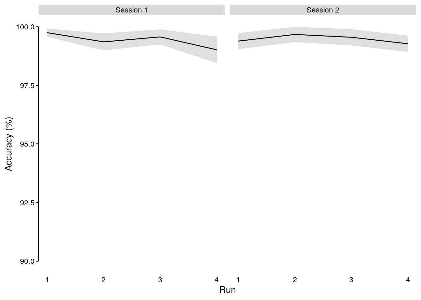
2.2.4.4 Source Data File Fig. S1c
dt_odd_behav_run_mean %>%
select(-num_subs, -mean_accuracy_z) %>%
write.csv(., file = file.path(path_sourcedata, "source_data_figure_s1c.csv"),
row.names = FALSE)2.2.4.5 Misses vs. false alarms
We calculate the mean frequency of misses (missed response to upside-down images) and false alarms (incorrect response to upright images):
dt_odd_behav_sdt_sub = dt_events %>%
# exclude participants performing below chance:
filter(!(subject %in% subjects_excluded)) %>%
# select only oddball condition and stimulus events:
filter(condition == "oddball" & trial_type == "stimulus") %>%
setDT(.) %>%
# create new variable with number of upside-down / upright stimuli per run:
.[, by = .(subject, session, run_session, stim_orient), ":=" (
num_orient = .N
)] %>%
# get the number of signal detection trial types for each run:
.[, by = .(subject, session, run_session, sdt_type), .(
num_trials = .N,
freq = .N/unique(num_orient)
)] %>%
# add missing values:
complete(nesting(subject, session, run_session), nesting(sdt_type),
fill = list(num_trials = 0, freq = 0)) %>%
transform(freq = freq * 100) %>%
filter(sdt_type %in% c("false alarm", "miss"))We run a LME model to test the effect of signal detection type (miss vs. false alarm), task run and session on the frequency of those events:
lme_odd_behav_sdt = lmer(
freq ~ sdt_type + run_session * session + (1 + run_session + session | subject),
data = subset(dt_odd_behav_sdt_sub), na.action = na.omit, control = lcctrl)
summary(lme_odd_behav_sdt)
anova(lme_odd_behav_sdt)
emmeans_results = emmeans(lme_odd_behav_sdt, list(pairwise ~ sdt_type))
emmeans_pvalues = round_pvalues(summary(emmeans_results[[2]])$p.value)
emmeans_results## Linear mixed model fit by REML. t-tests use Satterthwaite's method [
## lmerModLmerTest]
## Formula: freq ~ sdt_type + run_session * session + (1 + run_session +
## session | subject)
## Data: subset(dt_odd_behav_sdt_sub)
## Control: lcctrl
##
## REML criterion at convergence: 2164.6
##
## Scaled residuals:
## Min 1Q Median 3Q Max
## -2.3848 -0.2865 -0.1767 -0.0525 7.7856
##
## Random effects:
## Groups Name Variance Std.Dev. Corr
## subject (Intercept) 0.12419 0.3524
## run_session 0.09805 0.3131 0.37
## session 0.32394 0.5692 -0.94 -0.66
## Residual 2.21395 1.4879
## Number of obs: 576, groups: subject, 36
##
## Fixed effects:
## Estimate Std. Error df t value Pr(>|t|)
## (Intercept) 0.10130 0.48776 457.56239 0.208 0.8356
## sdt_typemiss 0.25175 0.12399 501.00009 2.030 0.0429 *
## run_session 0.06991 0.18296 442.67822 0.382 0.7026
## session 0.05953 0.31819 366.45275 0.187 0.8517
## run_session:session -0.01733 0.11090 501.00010 -0.156 0.8759
## ---
## Signif. codes: 0 '***' 0.001 '**' 0.01 '*' 0.05 '.' 0.1 ' ' 1
##
## Correlation of Fixed Effects:
## (Intr) sdt_ty rn_sss sessin
## sdt_typemss -0.127
## run_session -0.849 0.000
## session -0.925 0.000 0.736
## rn_sssn:sss 0.853 0.000 -0.909 -0.871
## Type III Analysis of Variance Table with Satterthwaite's method
## Sum Sq Mean Sq NumDF DenDF F value Pr(>F)
## sdt_type 9.1265 9.1265 1 501.00 4.1223 0.04285 *
## run_session 0.3232 0.3232 1 442.68 0.1460 0.70258
## session 0.0775 0.0775 1 366.45 0.0350 0.85169
## run_session:session 0.0541 0.0541 1 501.00 0.0244 0.87587
## ---
## Signif. codes: 0 '***' 0.001 '**' 0.01 '*' 0.05 '.' 0.1 ' ' 1
## $`emmeans of sdt_type`
## sdt_type emmean SE df lower.CL upper.CL
## false alarm 0.300 0.118 66.4 0.0656 0.535
## miss 0.552 0.118 66.4 0.3174 0.787
##
## Results are averaged over the levels of: session
## Degrees-of-freedom method: kenward-roger
## Confidence level used: 0.95
##
## $`pairwise differences of sdt_type`
## contrast estimate SE df t.ratio p.value
## false alarm - miss -0.252 0.124 466 -2.030 0.0429
##
## Results are averaged over the levels of: session
## Degrees-of-freedom method: kenward-roger2.2.4.6 Figure S1b
We plot the frequency of misses and false alarms as a function of task run and study session:
plot_odd_sdt = ggplot(data = dt_odd_behav_sdt_sub, mapping = aes(
y = as.numeric(freq), x = as.numeric(run_session),
fill = as.factor(sdt_type), color = as.factor(sdt_type))) +
stat_summary(geom = "bar", fun = mean, position = position_dodge(),
na.rm = TRUE) +
stat_summary(geom = "errorbar", fun.data = mean_se,
position = position_dodge(0.9), width = 0, color = "black") +
facet_wrap(~ as.factor(session), labeller = as_labeller(facet_labels_new)) +
geom_dotplot(
aes(group = interaction(run_session, session, sdt_type)),
binaxis = "y", stackdir = "center", stackratio = 0.2, alpha = 0.7,
inherit.aes = TRUE, binwidth = 0.2, position = position_dodge(),
color = "black") +
ylab("Frequency (%)") + xlab("Run") +
coord_capped_cart(left = "both", bottom = "both",
expand = TRUE, ylim = c(0, 15)) +
scale_fill_viridis(name = "Error", discrete = TRUE) +
scale_color_viridis(name = "Error", discrete = TRUE) +
theme(strip.text.x = element_text(margin = margin(b = 2, t = 2))) +
theme(legend.position = "top", legend.direction = "horizontal",
legend.justification = "center", legend.margin = margin(0, 0, 0, 0),
legend.box.margin = margin(t = 0, r = 0, b = -5, l = 0)) +
theme(axis.text = element_text(color = "black")) +
theme(axis.ticks.x = element_line(color = "white")) +
theme(axis.line.x = element_line(color = "white")) +
theme(axis.ticks.y = element_line(color = "black")) +
theme(axis.line.y = element_line(colour = "black"),
panel.grid.major = element_blank(),
panel.grid.minor = element_blank(),
panel.border = element_blank(),
panel.background = element_blank())
plot_odd_sdt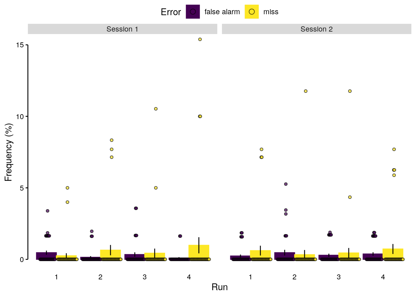
2.2.4.7 Source Data File Fig. S1b
dt_odd_behav_sdt_sub %>%
select(-num_trials) %>%
write.csv(., file = file.path(path_sourcedata, "source_data_figure_s1b.csv"),
row.names = FALSE)2.2.5 Sequence trials
2.2.5.1 Effect of sequence speed
We calculate the mean behavioral accuracy on sequence trials for each of the five sequence speeds (inter-stimulus intervals):
dt_seq_behav = dt_events %>%
# filter behavioral events data for sequence trials only:
filter(condition == "sequence") %>%
setDT(.) %>%
# create additional variables to describe each trial:
.[, by = .(subject, trial), ":=" (
trial_key_down = ifelse(any(key_down == 1, na.rm = TRUE), 1, 0),
trial_accuracy = ifelse(any(accuracy == 1, na.rm = TRUE), 1, 0),
trial_target_position = serial_position[which(target == 1)],
trial_speed = unique(interval_time[which(!is.na(interval_time))])
)] %>%
# filter for choice trials only:
filter(trial_type == "choice") %>%
setDT(.) %>%
# group speed conditions into fast and slow conditions:
mutate(speed = ifelse(trial_speed %in% c(2.048, 0.512), "slow", "fast")) %>%
# define variable factors of interest as numeric:
transform(trial_speed = as.numeric(trial_speed)) %>%
transform(trial_target_position = as.numeric(trial_target_position)) %>%
setDT(.)dt_seq_behav_speed = dt_seq_behav %>%
# filter out excluded subjects:
filter(!(subject %in% subjects_excluded)) %>%
setDT(.) %>%
# average accuracy for each participant:
.[, by = .(subject, trial_speed), .(
num_trials = .N,
mean_accuracy = mean(accuracy)
)] %>%
transform(mean_accuracy = mean_accuracy * 100) %>%
setDT(.) %>%
verify(all(num_trials == 15)) %>%
verify(.[, by = .(trial_speed), .(
num_subjects = .N
)]$num_subjects == 36) %>%
setorder(subject, trial_speed) %>%
mutate(trial_speed = as.numeric(trial_speed)) %>%
setDT(.)We run a LME model to test the effect of sequence speed (inter-stimulus interval) on mean behavioral accuracy on sequence trials:
lme_seq_behav = lmer(
mean_accuracy ~ trial_speed + (1 + trial_speed | subject),
data = dt_seq_behav_speed, na.action = na.omit, control = lcctrl)
summary(lme_seq_behav)
anova(lme_seq_behav)
emmeans_results = emmeans(lme_seq_behav, list(pairwise ~ trial_speed))
emmeans_pvalues = round_pvalues(summary(emmeans_results[[2]])$p.value)
emmeans_results
emmeans_pvalues## Linear mixed model fit by REML. t-tests use Satterthwaite's method [
## lmerModLmerTest]
## Formula: mean_accuracy ~ trial_speed + (1 + trial_speed | subject)
## Data: dt_seq_behav_speed
## Control: lcctrl
##
## REML criterion at convergence: 1245.4
##
## Scaled residuals:
## Min 1Q Median 3Q Max
## -2.8011 -0.4849 0.2106 0.6766 2.3025
##
## Random effects:
## Groups Name Variance Std.Dev. Corr
## subject (Intercept) 32.535 5.704
## trial_speed 3.969 1.992 -0.58
## Residual 44.342 6.659
## Number of obs: 180, groups: subject, 36
##
## Fixed effects:
## Estimate Std. Error df t value Pr(>|t|)
## (Intercept) 91.0872 1.1316 35.0000 80.495 <2e-16 ***
## trial_speed 1.5063 0.7287 35.0000 2.067 0.0462 *
## ---
## Signif. codes: 0 '***' 0.001 '**' 0.01 '*' 0.05 '.' 0.1 ' ' 1
##
## Correlation of Fixed Effects:
## (Intr)
## trial_speed -0.508
## Type III Analysis of Variance Table with Satterthwaite's method
## Sum Sq Mean Sq NumDF DenDF F value Pr(>F)
## trial_speed 189.49 189.49 1 35 4.2733 0.04617 *
## ---
## Signif. codes: 0 '***' 0.001 '**' 0.01 '*' 0.05 '.' 0.1 ' ' 1
## $`emmeans of trial_speed`
## trial_speed emmean SE df lower.CL upper.CL
## 0.557 91.9 0.989 35 89.9 93.9
##
## Degrees-of-freedom method: kenward-roger
## Confidence level used: 0.95
##
## $` of trial_speed`
## contrast estimate SE df z.ratio p.value
## (nothing) nonEst NA NA NA NA
##
## Degrees-of-freedom method: kenward-roger
##
## [1] "p = NA"We compare mean behavioral accuracy at each sequence speed level to the chancel level of 50%:
chance_level = 50
dt_seq_behav_mean = dt_seq_behav_speed %>%
# average across participants:
.[, by = .(trial_speed), {
ttest_results = t.test(
mean_accuracy, mu = chance_level, alternative = "greater")
list(
mean_accuracy = round(mean(mean_accuracy), digits = 2),
sd_accuracy = round(sd(mean_accuracy), digits = 2),
tvalue = round(ttest_results$statistic, digits = 2),
conf_lb = round(ttest_results$conf.int[1], digits = 2),
conf_ub = round(ttest_results$conf.int[2], digits = 2),
pvalue = ttest_results$p.value,
cohens_d = round((mean(mean_accuracy) - chance_level)/sd(mean_accuracy), 2),
df = ttest_results$parameter,
num_subs = .N,
sem_upper = mean(mean_accuracy) + (sd(mean_accuracy)/sqrt(.N)),
sem_lower = mean(mean_accuracy) - (sd(mean_accuracy)/sqrt(.N))
)}] %>%
verify(num_subs == 36) %>%
mutate(sem_range = sem_upper - sem_lower) %>%
mutate(pvalue_adjust = p.adjust(pvalue, method = "fdr")) %>%
mutate(pvalue_adjust_round = round_pvalues(pvalue_adjust))
# print paged table:
rmarkdown::paged_table(dt_seq_behav_mean)We calculate the reduction in mean behavioral accuracy comparing the fastest and slowest speed condition:
a = dt_seq_behav_mean$mean_accuracy[dt_seq_behav_mean$trial_speed == 2.048]
b = dt_seq_behav_mean$mean_accuracy[dt_seq_behav_mean$trial_speed == 0.032]
reduced_acc = round((1 - (b/a)) * 100, 2)
sprintf("reduction in accuracy: %.2f", reduced_acc)## [1] "reduction in accuracy: 5.73"2.2.5.2 Figure 1e
fig_seq_speed = ggplot(data = dt_seq_behav_speed, mapping = aes(
y = as.numeric(mean_accuracy), x = as.factor(as.numeric(trial_speed)*1000),
fill = as.factor(trial_speed), color = as.factor(trial_speed))) +
geom_bar(stat = "summary", fun = "mean") +
geom_dotplot(binaxis = "y", stackdir = "center", stackratio = 0.5,
color = "black", alpha = 0.5,
inherit.aes = TRUE, binwidth = 2) +
geom_errorbar(stat = "summary", fun.data = "mean_se", width = 0.0, color = "black") +
geom_hline(aes(yintercept = 50), linetype = "dashed", color = "black") +
ylab("Accuracy (%)") + xlab("Sequence speed (ms)") +
scale_fill_viridis(discrete = TRUE, guide = FALSE, option = "cividis") +
scale_color_viridis(discrete = TRUE, guide = FALSE, option = "cividis") +
coord_capped_cart(left = "both", bottom = "both", expand = TRUE, ylim = c(0, 100)) +
theme(plot.title = element_text(size = 12, face = "plain")) +
theme(axis.ticks.x = element_blank(), axis.line.x = element_blank()) +
ggtitle("Sequence") +
theme(plot.title = element_text(hjust = 0.5)) +
theme(axis.text = element_text(color = "black")) +
theme(axis.ticks.x = element_line(color = "white")) +
theme(axis.line.x = element_line(color = "white")) +
theme(axis.ticks.y = element_line(color = "black")) +
theme(axis.line.y = element_line(colour = "black"),
panel.grid.major = element_blank(),
panel.grid.minor = element_blank(),
panel.border = element_blank(),
panel.background = element_blank())
fig_seq_speed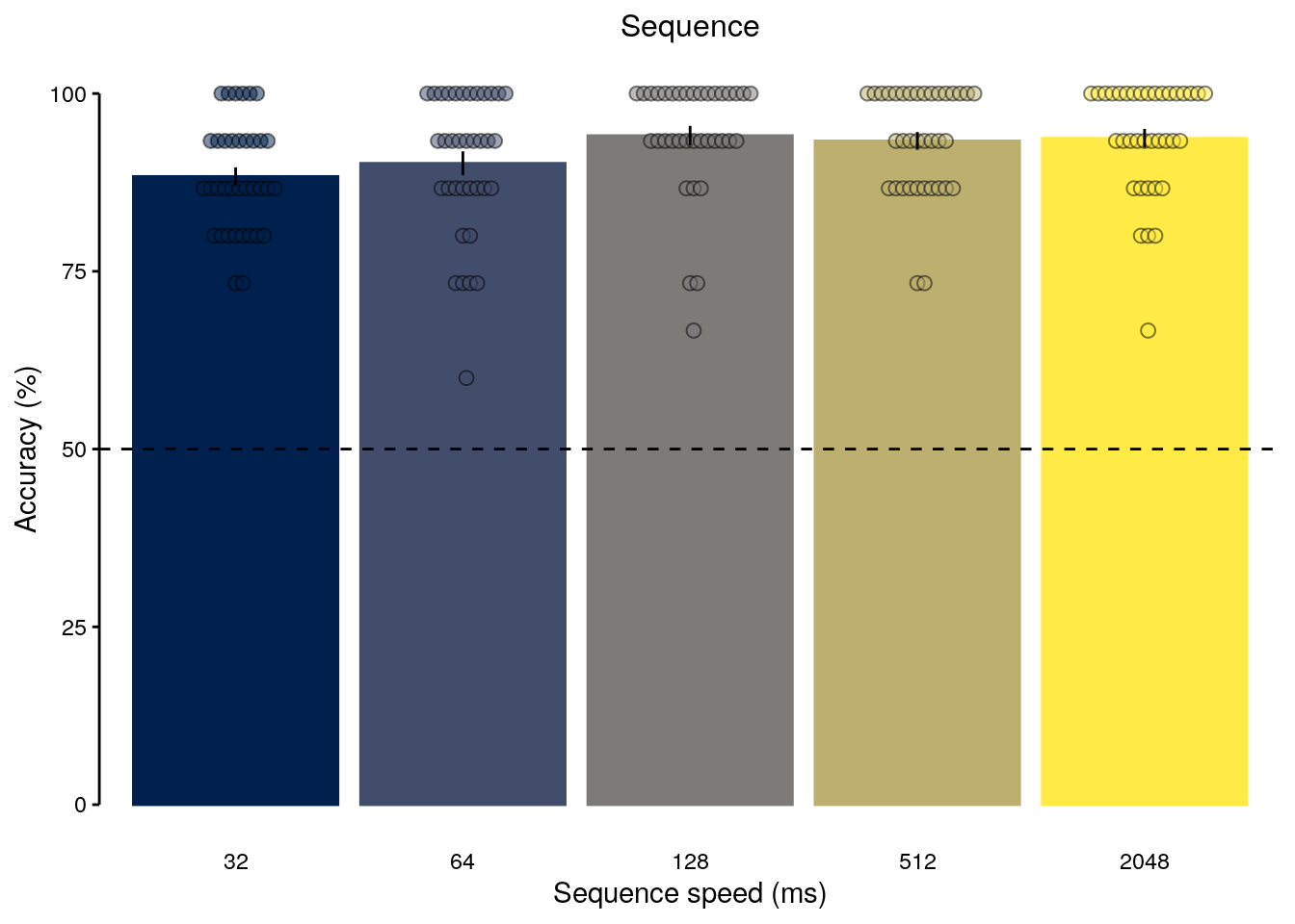
2.2.5.3 Source Data File Fig. 1e
dt_seq_behav_speed %>%
select(-num_trials) %>%
write.csv(., file = file.path(path_sourcedata, "source_data_figure_1e.csv"),
row.names = FALSE)2.2.5.4 Effect of target position
We calculate the mean behavioral accuracy on sequence trials for each of possible serial position of the target stimulus:
dt_seq_behav_position = dt_seq_behav %>%
# filter out excluded subjects:
filter(!(subject %in% subjects_excluded)) %>% setDT(.) %>%
# average accuracy for each participant:
.[, by = .(subject, trial_target_position), .(
num_trials = .N,
mean_accuracy = mean(accuracy)
)] %>%
verify(.[, by = .(trial_target_position), .(
num_subs = .N
)]$num_subs == 36) %>%
transform(mean_accuracy = mean_accuracy * 100) %>%
setorder(subject, trial_target_position)lme_seq_behav_position = lmer(
mean_accuracy ~ trial_target_position + (1 + trial_target_position | subject),
data = dt_seq_behav_position, na.action = na.omit, control = lcctrl)
summary(lme_seq_behav_position)## Linear mixed model fit by REML. t-tests use Satterthwaite's method [
## lmerModLmerTest]
## Formula: mean_accuracy ~ trial_target_position + (1 + trial_target_position |
## subject)
## Data: dt_seq_behav_position
## Control: lcctrl
##
## REML criterion at convergence: 1385.9
##
## Scaled residuals:
## Min 1Q Median 3Q Max
## -3.2760 -0.4809 0.1467 0.5073 2.1940
##
## Random effects:
## Groups Name Variance Std.Dev. Corr
## subject (Intercept) 221.205 14.873
## trial_target_position 8.402 2.899 -1.00
## Residual 102.478 10.123
## Number of obs: 180, groups: subject, 36
##
## Fixed effects:
## Estimate Std. Error df t value Pr(>|t|)
## (Intercept) 83.4370 3.0456 35.9399 27.396 < 2e-16 ***
## trial_target_position 2.2667 0.7197 42.0225 3.149 0.00301 **
## ---
## Signif. codes: 0 '***' 0.001 '**' 0.01 '*' 0.05 '.' 0.1 ' ' 1
##
## Correlation of Fixed Effects:
## (Intr)
## trl_trgt_ps -0.936anova(lme_seq_behav_position)## Type III Analysis of Variance Table with Satterthwaite's method
## Sum Sq Mean Sq NumDF DenDF F value Pr(>F)
## trial_target_position 1016.4 1016.4 1 42.022 9.9178 0.003011 **
## ---
## Signif. codes: 0 '***' 0.001 '**' 0.01 '*' 0.05 '.' 0.1 ' ' 12.2.5.5 Figure S1d
fig_seq_position = ggplot(data = dt_seq_behav_position, mapping = aes(
y = as.numeric(mean_accuracy), x = as.factor(trial_target_position),
fill = as.factor(trial_target_position), color = as.factor(trial_target_position))) +
geom_bar(stat = "summary", fun = "mean") +
geom_dotplot(binaxis = "y", stackdir = "center", stackratio = 0.5,
color = "black", alpha = 0.5,
inherit.aes = TRUE, binwidth = 2) +
geom_errorbar(stat = "summary", fun.data = "mean_se", width = 0.0, color = "black") +
geom_hline(aes(yintercept = 50), linetype = "dashed", color = "black") +
ylab("Accuracy (%)") + xlab("Target position") +
scale_fill_manual(values = color_events, guide = FALSE) +
scale_color_manual(values = color_events, guide = FALSE) +
coord_capped_cart(left = "both", bottom = "both", expand = TRUE, ylim = c(0, 100)) +
theme(axis.ticks.x = element_blank(), axis.line.x = element_blank()) +
theme(axis.text = element_text(color = "black")) +
theme(axis.ticks.x = element_line(color = "white")) +
theme(axis.line.x = element_line(color = "white")) +
theme(axis.ticks.y = element_line(color = "black")) +
theme(axis.line.y = element_line(colour = "black"),
panel.grid.major = element_blank(),
panel.grid.minor = element_blank(),
panel.border = element_blank(),
panel.background = element_blank())
fig_seq_position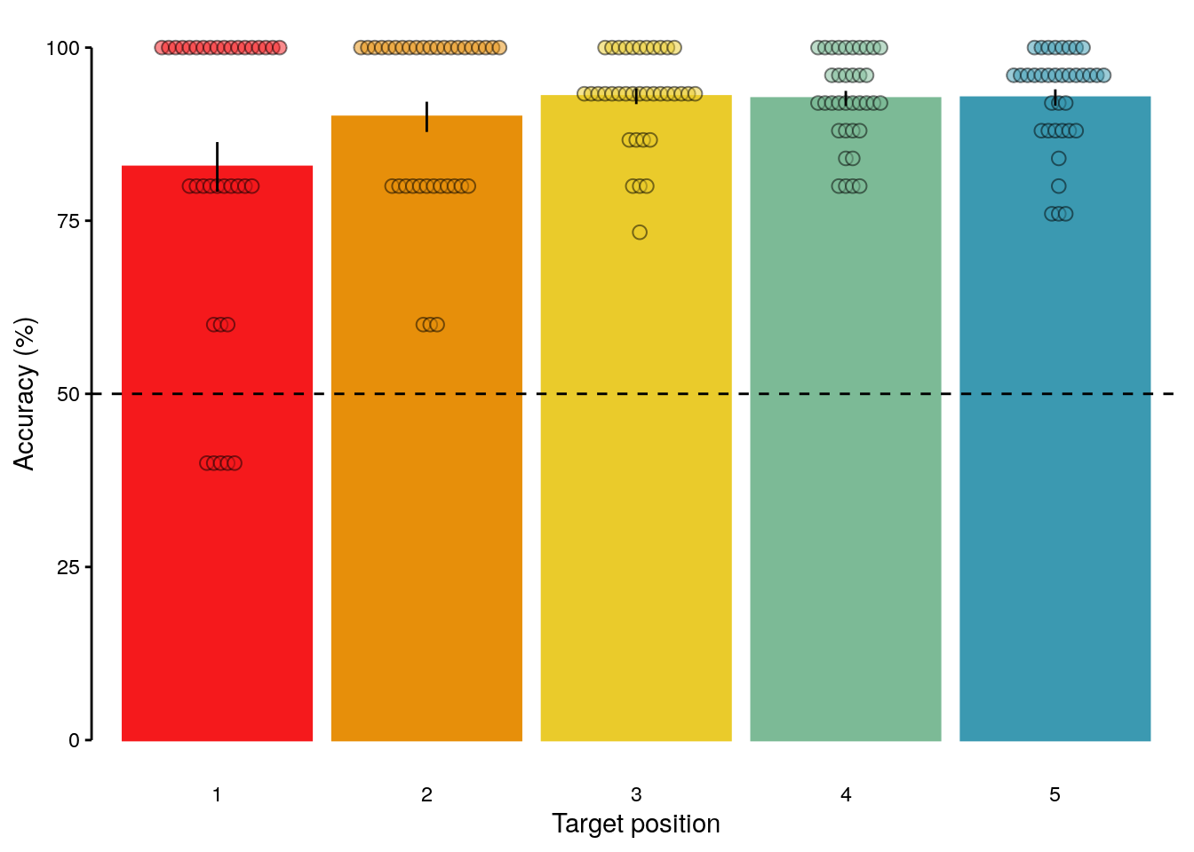
2.2.5.6 Source Data File Fig. S1d
dt_seq_behav_position %>%
select(-num_trials) %>%
write.csv(., file = file.path(path_sourcedata, "source_data_figure_s1d.csv"),
row.names = FALSE)2.2.6 Repetition trials
2.2.6.1 Mean accuracy
We calculate mean behavioral accuracy in repetition trials for each participant:
dt_rep_behav = dt_events %>%
# filter for repetition trials only:
filter(condition == "repetition") %>% setDT(.) %>%
# create additional variables to describe each trial:
.[, by = .(subject, trial), ":=" (
trial_key_down = ifelse(any(key_down == 1, na.rm = TRUE), 1, 0),
trial_accuracy = ifelse(any(accuracy == 1, na.rm = TRUE), 1, 0),
trial_target_position = serial_position[which(target == 1)],
trial_speed = unique(interval_time[which(!is.na(interval_time))])
)] %>%
# select only choice trials that contain the accuracy data:
filter(trial_type == "choice") %>% setDT(.) %>%
verify(all(trial_accuracy == accuracy)) %>%
# average across trials separately for each participant:
.[, by = .(subject, trial_target_position), .(
num_trials = .N,
mean_accuracy = mean(accuracy)
)] %>%
verify(all(num_trials == 5)) %>%
# transform mean accuracy into percent (%)
transform(mean_accuracy = mean_accuracy * 100) %>%
# check if accuracy values range between 0 and 100
verify(between(x = mean_accuracy, lower = 0, upper = 100)) %>%
mutate(interference = ifelse(
trial_target_position == 2, "fwd", trial_target_position)) %>%
transform(interference = ifelse(
trial_target_position == 9, "bwd", interference))We run separate one-sided one-sample t-tests to access if mean behavioral performance for every repetition condition differs from a 50% chance level:
chance_level = 50
dt_rep_behav_chance = dt_rep_behav %>%
# filter out excluded subjects:
filter(!(subject %in% subjects_excluded)) %>%
setDT(.) %>%
# average across participants:
.[, by = .(trial_target_position), {
ttest_results = t.test(
mean_accuracy, mu = chance_level, alternative = "greater")
list(
mean_accuracy = round(mean(mean_accuracy), digits = 2),
sd_accuracy = round(sd(mean_accuracy), digits = 2),
tvalue = round(ttest_results$statistic, digits = 2),
pvalue = ttest_results$p.value,
conf_lb = round(ttest_results$conf.int[1], digits = 2),
conf_ub = round(ttest_results$conf.int[2], digits = 2),
cohens_d = round((mean(mean_accuracy) - chance_level)/sd(mean_accuracy), 2),
df = ttest_results$parameter,
num_subs = .N,
sem_upper = mean(mean_accuracy) + (sd(mean_accuracy)/sqrt(.N)),
sem_lower = mean(mean_accuracy) - (sd(mean_accuracy)/sqrt(.N))
)}] %>% verify(num_subs == 36) %>%
mutate(sem_range = sem_upper - sem_lower) %>%
setDT(.) %>%
filter(trial_target_position %in% seq(2,9)) %>%
# create additional variable to label forward and backward interference:
mutate(interference = ifelse(
trial_target_position == 2, "fwd", trial_target_position)) %>%
transform(interference = ifelse(
trial_target_position == 9, "bwd", interference)) %>%
mutate(pvalue_adjust = p.adjust(pvalue, method = "fdr")) %>%
mutate(pvalue_adjust_round = round_pvalues(pvalue_adjust)) %>%
mutate(significance = ifelse(pvalue_adjust < 0.05, "*", "")) %>%
mutate(cohens_d = paste0("d = ", cohens_d, significance)) %>%
mutate(label = paste0(
trial_target_position - 1, "/", 10 - trial_target_position)) %>%
setDT(.) %>%
setorder(trial_target_position)
# print table:
rmarkdown::paged_table(dt_rep_behav_chance)2.2.6.2 Figure 1f
We plot the results of the forward and backward interference conditions:
plot_data = dt_rep_behav_chance %>% filter(trial_target_position %in% c(2,9))
fig_behav_rep = ggplot(data = plot_data, mapping = aes(
y = as.numeric(mean_accuracy), x = fct_rev(as.factor(interference)),
fill = as.factor(interference))) +
geom_bar(stat = "summary", fun = "mean") +
geom_dotplot(data = dt_rep_behav %>%
filter(!(subject %in% subjects_excluded)) %>%
filter(trial_target_position %in% c(2,9)) %>% setDT(.) %>%
.[, by = .(subject, interference), .(
mean_accuracy = mean(mean_accuracy)
)],
binaxis = "y", stackdir = "center", stackratio = 0.5,
color = "black", alpha = 0.5, inherit.aes = TRUE, binwidth = 2) +
geom_errorbar(aes(ymin = sem_lower, ymax = sem_upper), width = 0.0, color = "black") +
ylab("Accuracy (%)") + xlab("Interfererence") +
ggtitle("Repetition") +
theme(plot.title = element_text(hjust = 0.5)) +
scale_fill_manual(values = c("red", "dodgerblue"), guide = FALSE) +
coord_capped_cart(left = "both", bottom = "both", expand = TRUE, ylim = c(0,100)) +
theme(axis.ticks.x = element_blank(), axis.line.x = element_blank()) +
theme(plot.title = element_text(size = 12, face = "plain")) +
#scale_y_continuous(labels = label_fill(seq(0, 100, 12.5), mod = 2), breaks = seq(0, 100, 12.5)) +
geom_hline(aes(yintercept = 50), linetype = "dashed", color = "black") +
#geom_text(aes(y = as.numeric(mean_accuracy) + 10, label = pvalue_adjust_round), size = 3) +
theme(axis.text = element_text(color = "black")) +
theme(axis.ticks.x = element_line(color = "white")) +
theme(axis.line.x = element_line(color = "white")) +
theme(axis.ticks.y = element_line(color = "black")) +
theme(axis.line.y = element_line(colour = "black"),
panel.grid.major = element_blank(),
panel.grid.minor = element_blank(),
panel.border = element_blank(),
panel.background = element_blank())
fig_behav_rep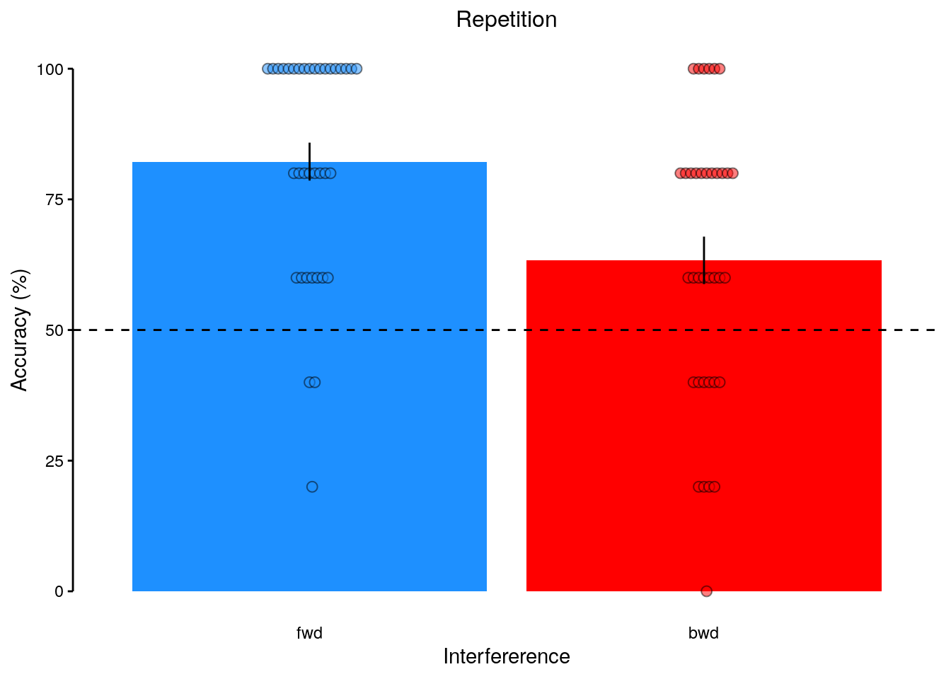
2.2.6.3 Source Data File Fig. 1f
dt_rep_behav %>%
select(-num_trials) %>%
write.csv(., file = file.path(path_sourcedata, "source_data_figure_1f.csv"),
row.names = FALSE)2.2.6.4 Figure S1e
We plot the results of all intermediate repetition conditions:
plot_data = dt_rep_behav_chance %>% filter(trial_target_position %in% seq(2,9))
plot_behav_rep_all = ggplot(data = plot_data, mapping = aes(
y = as.numeric(mean_accuracy), x = as.numeric(trial_target_position),
fill = as.numeric(trial_target_position))) +
geom_bar(stat = "identity") +
geom_dotplot(data = dt_rep_behav %>%
filter(!(subject %in% subjects_excluded)) %>%
filter(trial_target_position %in% seq(2,9)) %>% setDT(.) %>%
.[, by = .(subject, trial_target_position), .(
mean_accuracy = mean(mean_accuracy)
)],
aes(x = as.numeric(trial_target_position),
fill = as.numeric(trial_target_position),
group = as.factor(trial_target_position)),
binaxis = "y", stackdir = "center", stackratio = 0.5,
inherit.aes = TRUE, binwidth = 2, color = "black", alpha = 0.5) +
geom_errorbar(aes(ymin = sem_lower, ymax = sem_upper), width = 0.0, color = "black") +
geom_text(aes(y = as.numeric(mean_accuracy) + 7, label = cohens_d), size = 2.5) +
ylab("Accuracy (%)") + xlab("First / second item repetitions") +
scale_fill_gradient(low = "dodgerblue", high = "red", guide = FALSE) +
coord_capped_cart(left = "both", bottom = "both", expand = TRUE, ylim = c(0,100)) +
scale_x_continuous(labels = plot_data$label, breaks = seq(2, 9, 1)) +
geom_hline(aes(yintercept = 50), linetype = "dashed", color = "black") +
theme(axis.ticks.x = element_blank(), axis.line.x = element_blank()) +
theme(axis.text = element_text(color = "black")) +
theme(axis.ticks.x = element_line(color = "white")) +
theme(axis.line.x = element_line(color = "white")) +
theme(axis.ticks.y = element_line(color = "black")) +
theme(axis.line.y = element_line(colour = "black"),
panel.grid.major = element_blank(),
panel.grid.minor = element_blank(),
panel.border = element_blank(),
panel.background = element_blank())
plot_behav_rep_all
2.2.6.5 Source Data File Fig. S1e
dt_rep_behav %>%
select(-num_trials) %>%
write.csv(., file = file.path(path_sourcedata, "source_data_figure_s1e.csv"),
row.names = FALSE)ggsave(filename = "highspeed_plot_behavior_repetition_supplement.pdf",
plot = last_plot(), device = cairo_pdf, path = path_figures,
scale = 1, dpi = "retina", width = 5, height = 3, units = "in")We run a LME model to test the effect of repetition condition on mean behavioral accuracy in repetition trials:
lme_rep_behav_condition = lmer(
mean_accuracy ~ trial_target_position + (1 + trial_target_position|subject),
data = dt_rep_behav, na.action = na.omit, control = lcctrl)
summary(lme_rep_behav_condition)## Linear mixed model fit by REML. t-tests use Satterthwaite's method [
## lmerModLmerTest]
## Formula: mean_accuracy ~ trial_target_position + (1 + trial_target_position |
## subject)
## Data: dt_rep_behav
## Control: lcctrl
##
## REML criterion at convergence: 3287.6
##
## Scaled residuals:
## Min 1Q Median 3Q Max
## -3.3290 -0.6353 0.1102 0.7484 1.9475
##
## Random effects:
## Groups Name Variance Std.Dev. Corr
## subject (Intercept) 59.90 7.739
## trial_target_position 1.35 1.162 -0.02
## Residual 468.95 21.655
## Number of obs: 360, groups: subject, 40
##
## Fixed effects:
## Estimate Std. Error df t value Pr(>|t|)
## (Intercept) 87.7619 2.5538 39.0000 34.365 < 2e-16 ***
## trial_target_position -2.5976 0.3428 39.0000 -7.578 3.49e-09 ***
## ---
## Signif. codes: 0 '***' 0.001 '**' 0.01 '*' 0.05 '.' 0.1 ' ' 1
##
## Correlation of Fixed Effects:
## (Intr)
## trl_trgt_ps -0.643anova(lme_rep_behav_condition)## Type III Analysis of Variance Table with Satterthwaite's method
## Sum Sq Mean Sq NumDF DenDF F value Pr(>F)
## trial_target_position 26930 26930 1 39 57.426 3.493e-09 ***
## ---
## Signif. codes: 0 '***' 0.001 '**' 0.01 '*' 0.05 '.' 0.1 ' ' 12.2.7 Figure Main
We plot the figure for the main text:
2.2.8 Figure SI
We plot the figure for the supplementary information:
ggsave(filename = "wittkuhn_schuck_figure_s1.pdf",
plot = last_plot(), device = cairo_pdf, path = path_figures, scale = 1,
dpi = "retina", width = 8, height = 5)2.3 Participants
We analyze characteristics of the participants:
# read data table with participant information:
dt_participants <- do.call(rbind, lapply(Sys.glob(path_participants), fread))
# remove selected participants from the data table:
dt_participants = dt_participants %>%
filter(!(participant_id %in% subjects_excluded)) %>%
setDT(.)
base::table(dt_participants$sex)
round(sd(dt_participants$age), digits = 2)
base::summary(
dt_participants[, c("age", "digit_span", "session_interval"), with = FALSE])
round(sd(dt_participants$session_interval), digits = 2)##
## f m
## 20 16
## [1] 3.77
## age digit_span session_interval
## Min. :20.00 Min. : 9.00 Min. : 1.000
## 1st Qu.:22.00 1st Qu.:15.00 1st Qu.: 4.000
## Median :24.00 Median :16.00 Median : 7.500
## Mean :24.61 Mean :16.75 Mean : 9.167
## 3rd Qu.:26.00 3rd Qu.:19.00 3rd Qu.:13.250
## Max. :35.00 Max. :24.00 Max. :24.000
## [1] 6.142.4 Decoding on slow trials
2.4.1 Initialization
We load the data and relevant functions:
# find the path to the root of this project:
if (!requireNamespace("here")) install.packages("here")
if ( basename(here::here()) == "highspeed" ) {
path_root = here::here("highspeed-analysis")
} else {
path_root = here::here()
}
# create a list of participants to exclude based on behavioral performance:
sub_exclude <- c("sub-24", "sub-31", "sub-37", "sub-40")The next step is only evaluated during manual execution:
# source all relevant functions from the setup R script:
source(file.path(path_root, "code", "highspeed-analysis-setup.R"))2.4.2 Decoding accuracy
2.4.2.1 Mean decoding accuracy
We calculate the mean decoding accuracy:
calc_class_stim_acc <- function(data, mask_label) {
# calculate the mean decoding accuracy for each participant:
dt_odd_peak = data %>%
# select data for the oddball peak decoding
# leave out the redundant "other" class predictions:
filter(test_set == "test-odd_peak" & class != "other" & mask == mask_label) %>%
# filter out excluded participants:
filter(!(id %in% sub_exclude)) %>%
# only check classifier of stimulus presented on a given trial:
filter(class == stim) %>%
# calculate the decoding accuracy by comparing true and predicted label:
mutate(acc = 0) %>%
transform(acc = ifelse(pred_label == stim, 1, acc)) %>%
setDT(.) %>%
# calculate average decoding accuracy for every participant and classification:
.[, by = .(classification, id), .(
mean_accuracy = mean(acc) * 100,
num_trials = .N
)] %>%
verify(all(num_trials <= 480)) %>%
# verify if the number of participants matches:
verify(.[classification == "ovr", .(num_subs = .N)]$num_subs == 36)
return(dt_odd_peak)
}calc_max_prob_acc <- function(data, mask_label) {
dt_odd_peak <- data %>%
# select data for the oddball peak decoding
# leave out the redundant "other" class predictions:
filter(test_set == "test-odd_peak" & class != "other" & mask == mask_label) %>%
# filter out excluded participants:
filter(!(id %in% sub_exclude)) %>%
# calculate the decoding accuracy by comparing true and predicted label:
setDT(.) %>%
# calculate average decoding accuracy for every participant and classification:
.[, by = .(classification, id, trial, stim), .(
max_prob_label = class[which.max(probability)],
num_classes = .N
)] %>%
verify(num_classes == 5) %>%
.[, "acc" := ifelse(stim == max_prob_label, 1, 0)] %>%
.[, by = .(classification, id), .(
mean_accuracy = mean(acc) * 100,
num_trials = .N
)] %>%
verify(num_trials <= 480)
return(dt_odd_peak)
}We print the results for the decoding accuracy:
decoding_accuracy <- function(accuracy, alt_label){
# print average decoding accuracy:
print(sprintf("decoding accuracy: m = %0.2f %%", mean(accuracy)))
# print sd decoding accuracy:
print(sprintf("decoding accuracy: sd = %0.2f %%", sd(accuracy)))
# print range of decoding accuracy:
print(sprintf("decoding accuracy: range = %s %%",
paste(round(range(accuracy),0), collapse = "-")))
# define decoding accuracy baseline (should equal 20%):
acc_baseline = 100/5
print(sprintf("chance baseline = %d %%", acc_baseline))
# perform effect size (cohen`s d)
cohens_d = (mean(accuracy) - acc_baseline) / sd(accuracy)
print(sprintf("effect size (cohen's d) = %0.2f", cohens_d))
# perform shapiro-wilk test to test for normality of the data
print(shapiro.test(accuracy))
# perform one-sided one-sample t-test against baseline:
results = t.test(accuracy, mu = acc_baseline, alternative = alt_label)
print(results)
# perform one-sample wilcoxon test in case of non-normality of the data:
print(wilcox.test(accuracy, mu = acc_baseline, alternative = alt_label))
}#dt_odd_peak <- calc_class_stim_acc(data = dt_pred, mask_label = "cv")
#dt_odd_peak_hpc <- calc_class_stim_acc(data = dt_pred, mask_label = "cv_hpc")
dt_odd_peak <- calc_max_prob_acc(data = dt_pred, mask_label = "cv")
dt_odd_peak_hpc <- calc_max_prob_acc(data = dt_pred, mask_label = "cv_hpc")
decoding_accuracy(
accuracy = subset(dt_odd_peak, classification == "ovr")$mean_acc,
alt_label = "greater")
decoding_accuracy(
accuracy = subset(dt_odd_peak_hpc, classification == "ovr")$mean_accuracy,
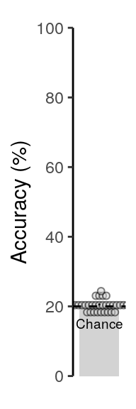
alt_label = "two.sided")## [1] "decoding accuracy: m = 69.22 %"
## [1] "decoding accuracy: sd = 11.18 %"
## [1] "decoding accuracy: range = 38-89 %"
## [1] "chance baseline = 20 %"
## [1] "effect size (cohen's d) = 4.40"
##
## Shapiro-Wilk normality test
##
## data: accuracy
## W = 0.94786, p-value = 0.08953
##
##
## One Sample t-test
##
## data: accuracy
## t = 26.409, df = 35, p-value < 2.2e-16
## alternative hypothesis: true mean is greater than 20
## 95 percent confidence interval:
## 66.07499 Inf
## sample estimates:
## mean of x
## 69.22417
##
##
## Wilcoxon signed rank exact test
##
## data: accuracy
## V = 666, p-value = 1.455e-11
## alternative hypothesis: true location is greater than 20
##
## [1] "decoding accuracy: m = 20.52 %"
## [1] "decoding accuracy: sd = 1.49 %"
## [1] "decoding accuracy: range = 17-24 %"
## [1] "chance baseline = 20 %"
## [1] "effect size (cohen's d) = 0.35"
##
## Shapiro-Wilk normality test
##
## data: accuracy
## W = 0.94782, p-value = 0.08928
##
##
## One Sample t-test
##
## data: accuracy
## t = 2.1007, df = 35, p-value = 0.04294
## alternative hypothesis: true mean is not equal to 20
## 95 percent confidence interval:
## 20.01755 21.02752
## sample estimates:
## mean of x
## 20.52254
##
##
## Wilcoxon signed rank test with continuity correction
##
## data: accuracy
## V = 440, p-value = 0.09424
## alternative hypothesis: true location is not equal to 202.4.2.2 Figure 2a / S2a
We plot the mean decoding accuracy in occipito-temporal and hippocampal data:
plot_odd_peak <- function(data) {
plot.odd = ggplot(data = data, aes(
x = "mean_acc", y = as.numeric(mean_accuracy))) +
geom_bar(stat = "summary", fun = "mean", fill = "lightgray") +
geom_dotplot(binaxis = "y", stackdir = "center", stackratio = 0.5,
color = "black", fill = "lightgray", alpha = 0.5,
inherit.aes = TRUE, binwidth = 2) +
geom_errorbar(stat = "summary", fun.data = "mean_se", width = 0.0, color = "black") +
ylab("Accuracy (%)") + xlab("Condition") +
geom_hline(aes(yintercept = 20), linetype = "dashed", color = "black") +
scale_y_continuous(labels = label_fill(seq(0, 100, 20), mod = 1),
breaks = seq(0, 100, 20)) +
coord_capped_cart(left = "both", expand = TRUE, ylim = c(0, 100)) +
theme(axis.ticks.x = element_blank(), axis.line.x = element_blank()) +
theme(axis.title.x = element_blank(), axis.text.x = element_blank()) +
annotate("text", x = 1, y = 15, label = "Chance", color = "black",
size = rel(2.5), family = "Helvetica", fontface = "plain") +
theme(panel.border = element_blank(), axis.line = element_line()) +
theme(axis.line = element_line(colour = "black"),
panel.grid.major = element_blank(),
panel.grid.minor = element_blank(),
panel.border = element_blank(),
panel.background = element_blank())
return(plot.odd)
}
fig_odd_peak <- plot_odd_peak(subset(dt_odd_peak, classification == "ovr"))
fig_odd_peak_hpc <- plot_odd_peak(subset(dt_odd_peak_hpc, classification == "ovr"))
fig_odd_peak; fig_odd_peak_hpc
2.4.2.3 Source Data File Fig. 2a
subset(dt_odd_peak, classification == "ovr") %>%
select(-num_trials, -classification) %>%
write.csv(., file = file.path(path_sourcedata, "source_data_figure_2a.csv"),
row.names = FALSE)2.4.2.4 Source Data File Fig. S2a
subset(dt_odd_peak_hpc, classification == "ovr") %>%
select(-num_trials, -classification) %>%
write.csv(., file = file.path(path_sourcedata, "source_data_figure_s2a.csv"),
row.names = FALSE)2.4.3 Fold-wise decoding accuracy
We calculate the mean decoding accuracy for each of the eight folds of the cross-validation procedure:
dt_odd_peak_run = dt_pred %>%
# select data for the oddball peak decoding
# leave out the redundant "other" class predictions:
filter(test_set == "test-odd_peak" & class != "other" & mask == "cv") %>%
# filter out excluded participants:
filter(!(id %in% sub_exclude)) %>%
setDT(.) %>%
# calculate average decoding accuracy for every participant and classification:
.[, by = .(classification, id, run_study, trial, stim), .(
max_prob_label = class[which.max(probability)],
num_classes = .N
)] %>%
# check if there are five classifier predictions per trial:
verify(num_classes == 5) %>%
# determine accuracy if label with highest probability matches stimulus:
.[, "accuracy" := ifelse(stim == max_prob_label, 1, 0)]
# print results table:
rmarkdown::paged_table(dt_odd_peak_run)# calculate average decoding accuracy for every participant and classification:
dt_odd_peak_run_mean <- dt_odd_peak_run %>%
.[, by = .(classification, id, run_study), .(
mean_accuracy = mean(accuracy) * 100,
num_trials = length(unique(trial))
)] %>%
# verify if the number of participants matches for every classification and run:
verify(.[, by = .(classification, run_study),
.(num_subs = .N)]$num_subs == 36) %>%
setorder(., classification, id, run_study)
# print the table:
rmarkdown::paged_table(dt_odd_peak_run_mean)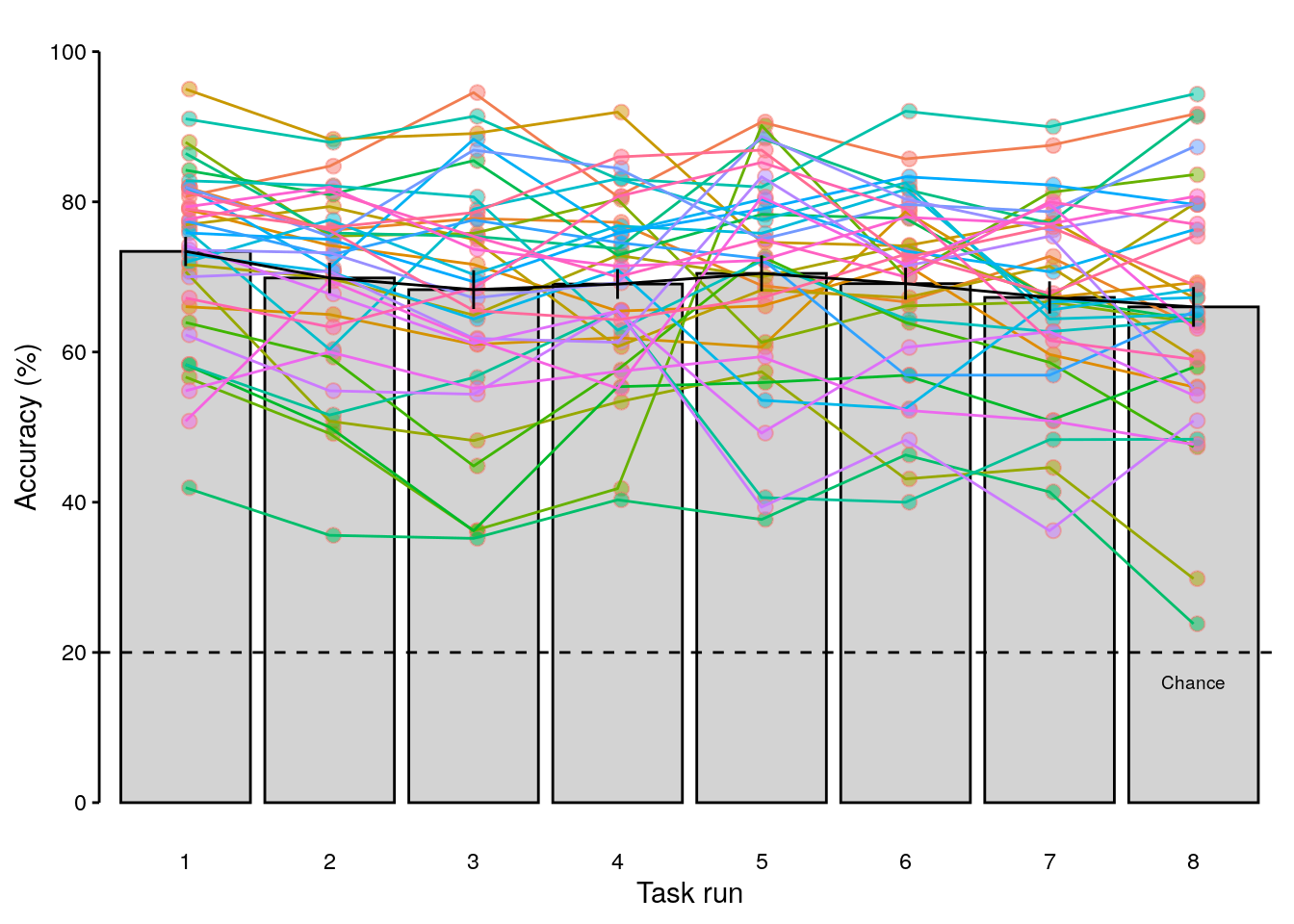
lme_odd_peak_run <- lmerTest::lmer(
mean_accuracy ~ run_study + (1 | id), control = lcctrl,
data = subset(dt_odd_peak_run_mean, classification == "ovr")
)
summary(lme_odd_peak_run)
anova(lme_odd_peak_run)
emmeans_results = emmeans(lme_odd_peak_run, list(pairwise ~ run_study))
emmeans_results## Linear mixed model fit by REML. t-tests use Satterthwaite's method [
## lmerModLmerTest]
## Formula: mean_accuracy ~ run_study + (1 | id)
## Data: subset(dt_odd_peak_run_mean, classification == "ovr")
## Control: lcctrl
##
## REML criterion at convergence: 2081.6
##
## Scaled residuals:
## Min 1Q Median 3Q Max
## -3.3758 -0.6237 0.0020 0.6078 3.1304
##
## Random effects:
## Groups Name Variance Std.Dev.
## id (Intercept) 117.30 10.830
## Residual 63.38 7.961
## Number of obs: 288, groups: id, 36
##
## Fixed effects:
## Estimate Std. Error df t value Pr(>|t|)
## (Intercept) 73.400 2.240 70.879 32.764 < 2e-16 ***
## run_study2 -3.538 1.876 245.000 -1.885 0.060551 .
## run_study3 -5.096 1.876 245.000 -2.716 0.007079 **
## run_study4 -4.348 1.876 245.000 -2.317 0.021318 *
## run_study5 -2.934 1.876 245.000 -1.564 0.119200
## run_study6 -4.294 1.876 245.000 -2.288 0.022970 *
## run_study7 -6.131 1.876 245.000 -3.268 0.001240 **
## run_study8 -7.391 1.876 245.000 -3.939 0.000107 ***
## ---
## Signif. codes: 0 '***' 0.001 '**' 0.01 '*' 0.05 '.' 0.1 ' ' 1
##
## Correlation of Fixed Effects:
## (Intr) rn_st2 rn_st3 rn_st4 rn_st5 rn_st6 rn_st7
## run_study2 -0.419
## run_study3 -0.419 0.500
## run_study4 -0.419 0.500 0.500
## run_study5 -0.419 0.500 0.500 0.500
## run_study6 -0.419 0.500 0.500 0.500 0.500
## run_study7 -0.419 0.500 0.500 0.500 0.500 0.500
## run_study8 -0.419 0.500 0.500 0.500 0.500 0.500 0.500
## Type III Analysis of Variance Table with Satterthwaite's method
## Sum Sq Mean Sq NumDF DenDF F value Pr(>F)
## run_study 1239.3 177.04 7 245 2.7936 0.008175 **
## ---
## Signif. codes: 0 '***' 0.001 '**' 0.01 '*' 0.05 '.' 0.1 ' ' 1
## $`emmeans of run_study`
## run_study emmean SE df lower.CL upper.CL
## 1 73.4 2.24 70.9 68.9 77.9
## 2 69.9 2.24 70.9 65.4 74.3
## 3 68.3 2.24 70.9 63.8 72.8
## 4 69.1 2.24 70.9 64.6 73.5
## 5 70.5 2.24 70.9 66.0 74.9
## 6 69.1 2.24 70.9 64.6 73.6
## 7 67.3 2.24 70.9 62.8 71.7
## 8 66.0 2.24 70.9 61.5 70.5
##
## Degrees-of-freedom method: kenward-roger
## Confidence level used: 0.95
##
## $`pairwise differences of run_study`
## contrast estimate SE df t.ratio p.value
## 1 - 2 3.5379 1.88 245 1.885 0.5622
## 1 - 3 5.0962 1.88 245 2.716 0.1227
## 1 - 4 4.3480 1.88 245 2.317 0.2885
## 1 - 5 2.9339 1.88 245 1.564 0.7715
## 1 - 6 4.2938 1.88 245 2.288 0.3043
## 1 - 7 6.1312 1.88 245 3.268 0.0268
## 1 - 8 7.3910 1.88 245 3.939 0.0027
## 2 - 3 1.5584 1.88 245 0.831 0.9912
## 2 - 4 0.8101 1.88 245 0.432 0.9999
## 2 - 5 -0.6039 1.88 245 -0.322 1.0000
## 2 - 6 0.7560 1.88 245 0.403 0.9999
## 2 - 7 2.5934 1.88 245 1.382 0.8647
## 2 - 8 3.8532 1.88 245 2.053 0.4482
## 3 - 4 -0.7482 1.88 245 -0.399 0.9999
## 3 - 5 -2.1623 1.88 245 -1.152 0.9442
## 3 - 6 -0.8024 1.88 245 -0.428 0.9999
## 3 - 7 1.0350 1.88 245 0.552 0.9993
## 3 - 8 2.2948 1.88 245 1.223 0.9245
## 4 - 5 -1.4140 1.88 245 -0.754 0.9951
## 4 - 6 -0.0541 1.88 245 -0.029 1.0000
## 4 - 7 1.7832 1.88 245 0.950 0.9806
## 4 - 8 3.0430 1.88 245 1.622 0.7368
## 5 - 6 1.3599 1.88 245 0.725 0.9962
## 5 - 7 3.1973 1.88 245 1.704 0.6847
## 5 - 8 4.4571 1.88 245 2.375 0.2582
## 6 - 7 1.8374 1.88 245 0.979 0.9770
## 6 - 8 3.0972 1.88 245 1.651 0.7189
## 7 - 8 1.2598 1.88 245 0.671 0.9976
##
## Degrees-of-freedom method: kenward-roger
## P value adjustment: tukey method for comparing a family of 8 estimates2.5 Single-trial decoding time courses
We calculate the multivariate decoding time courses on single slow trials:
dt_odd_long_sub = dt_pred %>%
# select data for the oddball long decoding
# leave out the redundant "other" class predictions:
filter(test_set == "test-odd_long" & class != "other" & mask == "cv") %>%
# filter out excluded participants:
filter(!(id %in% sub_exclude)) %>% setDT(.) %>%
# average across stimuli and runs for each participant
# create an index for the true stimulus presented on each trial:
.[, by = .(classification, id, seq_tr, class, stim), .(
num = .N,
mean_prob = mean(probability * 100),
current_stim = as.numeric(class == unique(stim))
)]
dt_odd_long_mean = dt_odd_long_sub %>%
# average across participants:
.[, by = .(classification, seq_tr, class, stim, current_stim), .(
mean_prob = mean(mean_prob),
num_subs = .N,
sem_upper = (mean(mean_prob) + (sd(mean_prob)/sqrt(.N))),
sem_lower = (mean(mean_prob) - (sd(mean_prob)/sqrt(.N)))
)] %>%
# create an additional variable that expresses time in seconds:
mutate(time = (seq_tr - 1) * 1.25) %>%
# check if the number of participants is correct:
verify(all(num_subs == 36))2.5.0.1 Figure 2b
We plot the single-trial multi-variate decoding time courses on slow trials:
plot.odd.long = ggplot(data = subset(dt_odd_long_mean, classification == "ovr"), aes(
x = as.factor(seq_tr), y = as.numeric(mean_prob))) +
facet_wrap(~ as.factor(stim)) +
geom_line(data = subset(dt_odd_long_sub, classification == "ovr"), aes(
group = as.factor(interaction(id, class)), color = fct_rev(as.factor(current_stim))), alpha = 0.0) +
geom_line(data = subset(dt_odd_long_sub, classification == "ovr" & current_stim == 0), aes(
group = as.factor(interaction(id, class)), color = fct_rev(as.factor(current_stim))), alpha = 0.3) +
geom_line(data = subset(dt_odd_long_sub, classification == "ovr" & current_stim == 1), aes(
group = as.factor(interaction(id, class)), color = fct_rev(as.factor(current_stim))), alpha = 0.3) +
geom_ribbon(
data = subset(dt_odd_long_mean, classification == "ovr"),
aes(ymin = sem_lower, ymax = sem_upper, fill = fct_rev(as.factor(current_stim)),
group = as.factor(class)), alpha = 0.0, color = NA) +
geom_line(
data = subset(dt_odd_long_mean, classification == "ovr", alpha = 0),
aes(color = fct_rev(as.factor(current_stim)), group = as.factor(class))) +
geom_ribbon(
data = subset(dt_odd_long_mean, classification == "ovr" & current_stim == 1),
aes(ymin = sem_lower, ymax = sem_upper, fill = fct_rev(as.factor(current_stim)),
group = as.factor(class)), alpha = 0.3, color = NA) +
geom_line(
data = subset(dt_odd_long_mean, classification == "ovr" & current_stim == 1),
aes(color = fct_rev(as.factor(current_stim)), group = as.factor(class))) +
ylab("Probability (%)") + xlab("Time from stimulus onset (TRs)") +
scale_fill_manual(name = "Classified class", values = c("black", "lightgray"), labels = c("true", "other")) +
scale_color_manual(name = "Classified class", values = c("black", "lightgray"), labels = c("true", "other")) +
coord_capped_cart(left = "both", bottom = "both", expand = TRUE, ylim = c(0, 80)) +
theme(legend.position = c(1, 0), legend.justification = c(1, 0)) +
#theme(legend.position = c(0.95, 0.8), legend.justification = c(1, 0)) +
#theme(legend.title = element_text(size = 8), legend.text = element_text(size = 8)) +
#theme(legend.key.size = unit(0.7, "line")) +
scale_x_discrete(labels = label_fill(seq(0, 7, 1), mod = 1), breaks = seq(0, 7, 1)) +
guides(color = guide_legend(ncol = 2), fill = guide_legend(ncol = 2)) +
theme(strip.text.x = element_text(margin = margin(b = 2, t = 2))) +
theme(panel.border = element_blank(), axis.line = element_line()) +
theme(axis.line = element_line(colour = "black"),
panel.grid.major = element_blank(),
panel.grid.minor = element_blank(),
panel.border = element_blank(),
panel.background = element_blank())
#theme(strip.text.x = element_blank())
plot.odd.long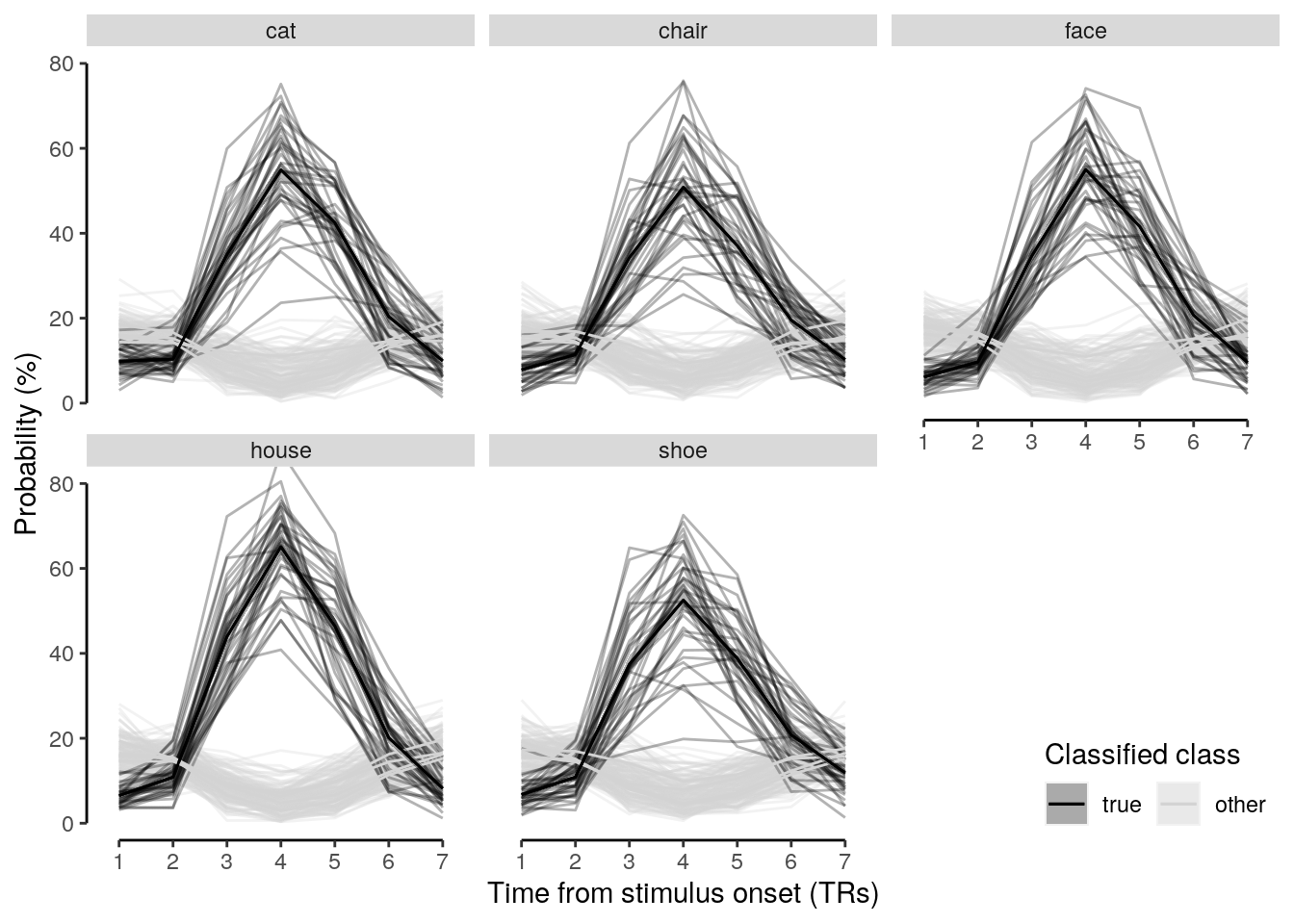
2.5.0.2 Source Data File Fig. 2b
subset(dt_odd_long_sub, classification == "ovr") %>%
select(-num, -classification) %>%
write.csv(., file = file.path(path_sourcedata, "source_data_figure_2b.csv"),
row.names = FALSE)We compare the mean classification probability of the current stimulus versus the mean of all other stimuli for each TR:
dt_odd_long_mean_stat = dt_pred %>%
# select data for the oddball long decoding
# leave out the redundant "other" class predictions:
filter(test_set == "test-odd_long" & class != "other" & mask == "cv") %>%
setDT(.) %>%
# filter out excluded participants:
filter(!(id %in% sub_exclude)) %>% setDT(.) %>%
# average across stimuli and runs for each participant
# create a new variable that indicated whether stimulus is current or not:
.[, by = .(classification, id, seq_tr, class, stim), .(
num_stim = .N,
mean_prob = mean(probability * 100),
stim_type = ifelse(class == unique(stim), "current", "other")
)] %>%
verify(num_stim <= 96) %>%
# average across stimulus type:
.[, by = .(classification, id, seq_tr, stim, stim_type), .(
num_class = .N,
mean_prob = mean(mean_prob)
)] %>%
verify(num_class %in% c(1, 4)) %>%
select(., -num_class) %>%
# turn into wide format:
spread(key = stim_type, value = mean_prob) %>% setDT(.) %>%
# calculate a paired t-test at every TR for each unique stimulus to
# compare probability of the current vs. the mean other class probabilities:
.[, by = .(classification, seq_tr, stim), {
results = t.test(current, other, paired = TRUE, alternative = "two.sided")
list(
tvalue = results$statistic,
df = results$parameter,
pvalue = results$p.value,
cohens_d = (mean(current) - mean(other)) / sd(current - other),
num_subs = .N,
mean_current = mean(current),
mean_other = mean(other),
pvalue_round = round_pvalues(results$p.value)
)
}] %>%
# ajdust the p-value for multiple comparisons using Bonferroni correction:
.[, by = .(classification), ":=" (
num_comp = .N,
pvalue_adjust = p.adjust(pvalue, method = "bonferroni", n = .N)
)] %>%
# check if correction was done for 5 (stimuli) by 7 (TRs) = 35 comparisons:
verify(all(num_comp == 5 * 7)) %>%
# verify if number of participants matches:
verify(all(num_subs == 36)) %>%
# check if degrees-of-freedom = n - 1
verify(all(df == num_subs - 1)) %>%
# round the bonferroni-adjusted p-values for clarity:
mutate(pvalue_adjust_round = round_pvalues(pvalue_adjust)) %>%
# sort the datatable according to classification, stimulus and TR:
setorder(., classification, stim, seq_tr) %>%
# only look at the fourth TR where probabilities are expected to peak
filter(seq_tr == 4 & classification == "ovr")
# print the data table:
rmarkdown::paged_table(dt_odd_long_mean_stat)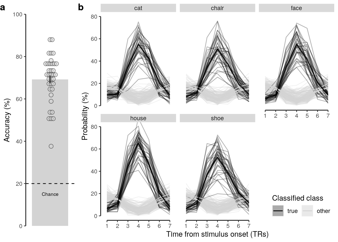
2.6 Response functions
2.6.1 Define response functions
We define the sine wave response function:
sine_truncated <- function(params, time) {
if (!is.list(params)) {
params = as.list(params)
names(params) = c('frequency', 'amplitude', 'shift', 'baseline')
}
y = rep(0, 13)
y = params$amp/2 * sin(2*pi*params$freq*time - 2*pi*params$freq*params$shift - 0.5*pi) + params$baseline + params$amp/2
# flatten response function after one cycle:
y[time < (params$shift)] = params$baseline
y[time > (params$shift + 1/params$freq)] = params$baseline
return(y)
}We define a function to evaluate during optimization:
sine_truncated_eval = function(params, time, data) {
y = sine_truncated(params, time)
SSE = sum((data - y)^2)
return(SSE)
}2.6.2 Mean parameters
We calculate the multivariate decoding time courses for each stimulus class:
# calculate mean probability for every stimulus for every TR:
dt_odd_long_mean_class = dt_pred %>%
# filter for oddball long predictions and only select ovr classifier:
filter(test_set == "test-odd_long" & class != "other" &
classification == "ovr" & mask == "cv") %>%
# filter out excluded participants:
filter(!(id %in% sub_exclude)) %>% setDT(.) %>%
# select only predictions for the class currently shown on any given trial:
filter(class == stim) %>% setDT(.) %>%
# average the probability across trials
.[, by = .(id, classification, stim, seq_tr), .(
mean_probability = mean(probability, na.rm = TRUE)
)]We fit the truncated sine wave response function to data from every participant:
# set optimization parameters:
opts = list("algorithm" = "NLOPT_LN_COBYLA", "xtol_rel" = 1.0e-8, "maxeval" = 1.0e+5)
default_params = c(0.2, 0.6, 0, 0.1)
lower_bounds = c(0.01, 0.1, 0, 0)
upper_bounds = c(0.5, 1, 5, 0.3)
time = 0:6dt_odd_long_fit = dt_odd_long_mean_class %>%
# fit the truncated sine wave to probabilities of every decoding timecourse:
.[, by = .(id, classification, stim), {
res <- nloptr(
x0 = default_params, eval_f = sine_truncated_eval, time = time,
data = mean_probability, lb = lower_bounds, ub = upper_bounds, opts = opts)
list(
num_trs = .N,
frequency = res$solution[1],
wavelength = 1/res$solution[1],
amplitude = res$solution[2],
shift = res$solution[3],
baseline = res$solution[4],
params = list(res$solution)
)}] %>%
verify(all(num_trs == length(time)))
# print the mean model parameters:
summary(dt_odd_long_fit[, c("frequency", "wavelength", "amplitude", "shift", "baseline")])
# calculate the mean parameters across all participants to be used later:
mean_parameters = dt_odd_long_fit %>%
# average the fitted parameters across participants:
.[, by = .(classification), .(
mean_freq = mean(frequency),
mean_wavelength = mean(wavelength),
mean_amplitude = mean(amplitude),
mean_shift = mean(shift),
mean_baseline = mean(baseline)
)]## frequency wavelength amplitude shift
## Min. :0.1307 Min. :2.000 Min. :0.1000 Min. :0.0000
## 1st Qu.:0.1776 1st Qu.:4.711 1st Qu.:0.3982 1st Qu.:0.4021
## Median :0.1942 Median :5.149 Median :0.4860 Median :0.5590
## Mean :0.1962 Mean :5.239 Mean :0.4858 Mean :0.5640
## 3rd Qu.:0.2123 3rd Qu.:5.630 3rd Qu.:0.5907 3rd Qu.:0.7087
## Max. :0.5000 Max. :7.651 Max. :0.8667 Max. :2.4777
## baseline
## Min. :0.02556
## 1st Qu.:0.06147
## Median :0.07928
## Mean :0.08081
## 3rd Qu.:0.09918
## Max. :0.15975We fit the sine response function for every participant using individual parameters:
dt_odd_long_fit_single = dt_odd_long_fit %>%
# calculate a sine-wave respone function timecourse for every participant:
.[, by = .(id, classification, stim), .(
csine = sine_truncated(params = unlist(params), seq(0, 6, 0.1))
)] %>%
# add a counter that is used for plotting below:
.[, by = .(classification, id, stim), ":=" (
t = seq(0, 6, 0.1))]2.6.2.1 Figure S4a
We plot the single sine wave fits for three example participants (supplement):
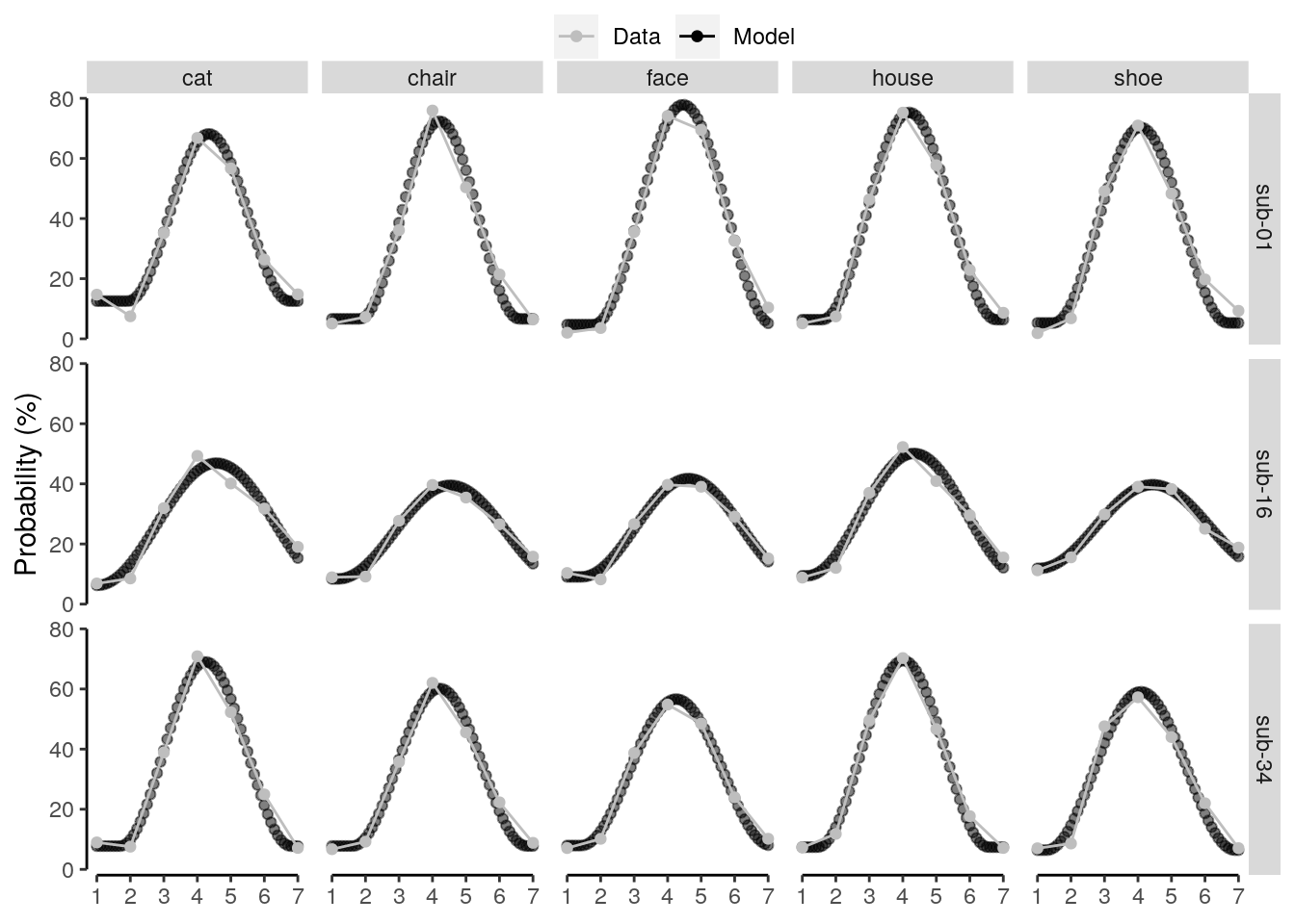
2.6.2.2 Source Data File Fig. S4a
dt_odd_long_mean_class %>%
select(-classification) %>%
write.csv(., file = file.path(path_sourcedata, "source_data_figure_s4a.csv"),
row.names = FALSE)We calculate the mean shape of the sine wave response function across participants:
dt_odd_long_fit_mean = dt_odd_long_fit %>%
# average the fitting parameters across participants:
.[, by = .(classification, stim), .(
num_subs = .N,
mean_freq = mean(frequency),
mean_amplitude = mean(amplitude),
mean_shift = mean(shift),
mean_baseline = mean(baseline)
)] %>% verify(all(num_subs == 36)) %>%
.[, by = .(classification, stim), .(
csine = sine_truncated(params = c(mean_freq, mean_amplitude, mean_shift, mean_baseline),
seq(0, 6, 0.1)))] %>%
.[, by = .(classification, stim), ":=" (
t = seq(0, 6, 0.1))]2.6.2.3 Figure S4b
fig_s2 = ggplot(data = dt_odd_long_mean_class) +
geom_line(data = dt_odd_long_mean_class,
aes(x = (seq_tr - 1), y = mean_probability * 100, group = as.factor(id),
color = "Data"), alpha = 0.3) +
geom_line(data = dt_odd_long_fit_mean, aes(x = t, y = csine * 100, color = "Model"),
size = 1) +
facet_wrap(~ as.factor(stim), nrow = 1) +
coord_capped_cart(left = "both", bottom = "both", ylim = c(0, 80)) +
xlab("Time from stimulus onset (in TRs)") + ylab("Probability (%)") +
scale_colour_manual(name = "", values = c("gray", "black"), guide = FALSE) +
scale_x_continuous(labels = label_fill(seq(1, 7, 1), mod = 1), breaks = seq(0, 6, 1)) +
#theme(plot.margin = unit(c(t = 1, r = 1, b = 1, l = 1), "pt")) +
theme(legend.position = "bottom", legend.direction = "horizontal",
legend.justification = "center", legend.margin = margin(0, 0, 0, 0),
legend.box.margin = margin(t = -10, r = 0, b = 0, l = 0)) +
theme(strip.text = element_text(margin = margin(b = 2, t = 2, r = 2, l = 2))) +
theme(axis.line = element_line(colour = "black"),
panel.grid.major = element_blank(),
panel.grid.minor = element_blank(),
panel.border = element_blank(),
panel.background = element_blank())
fig_s2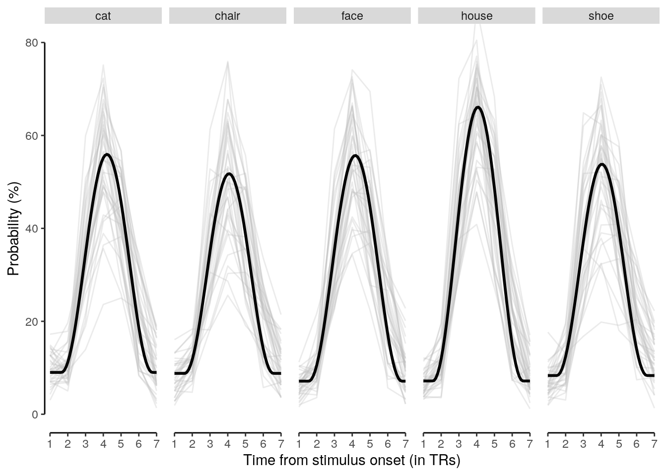
2.6.2.4 Source Data File Fig. S4b
dt_odd_long_mean_class %>%
select(-classification) %>%
write.csv(., file = file.path(path_sourcedata, "source_data_figure_s4b.csv"),
row.names = FALSE)2.6.2.5 Figure S4
plot_grid(fig_s1, fig_s2, nrow = 2, ncol = 1, hjust = c(0, 0),
rel_heights = c(4, 2), labels = c("a", "b"), label_fontface = "bold")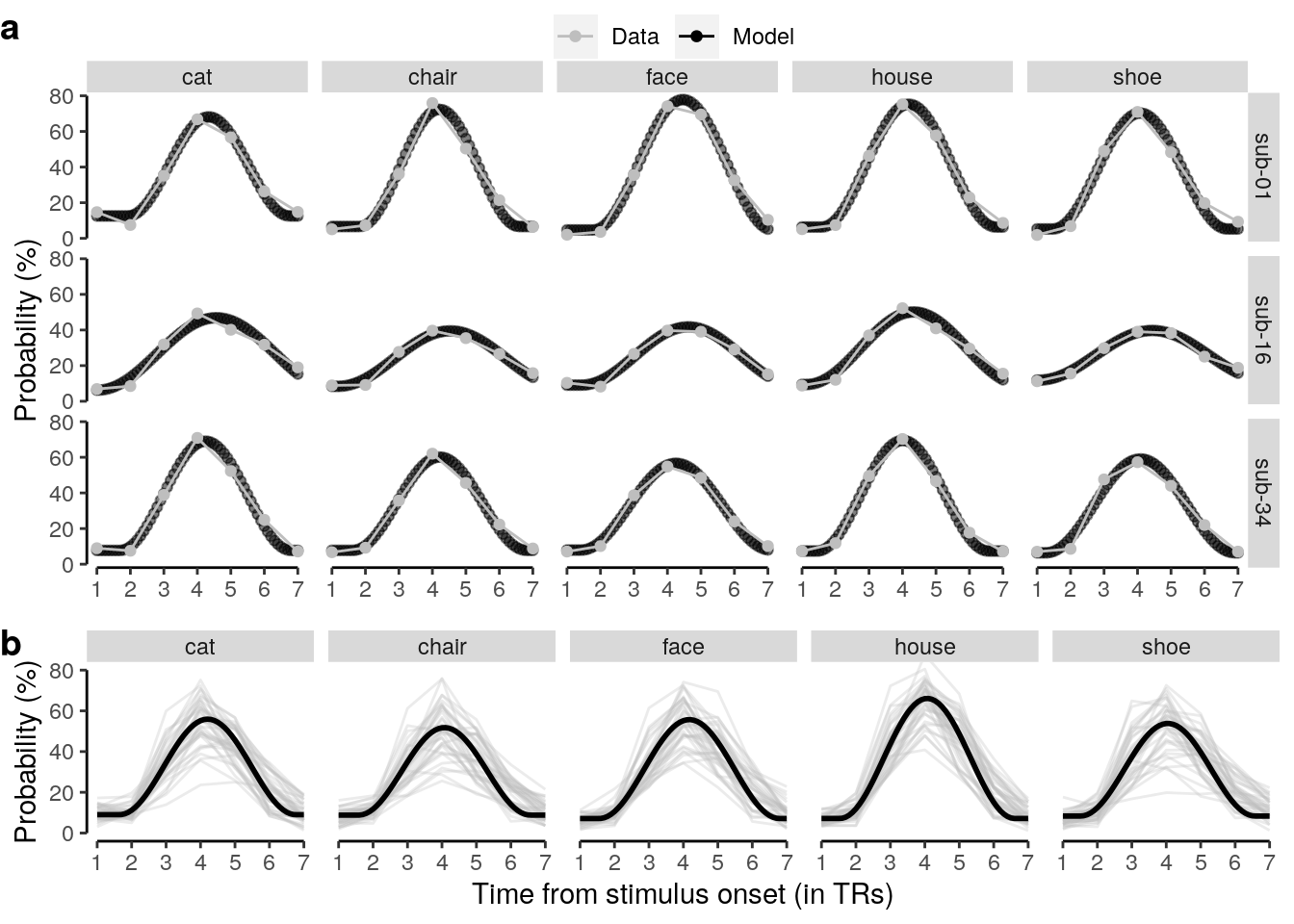
We evaluate the response function for two time-shifted events:
# horizontal phase shift (in TRs) that will be added to the second sine wave:
add_shift = 0.5
time = seq(0, 8, 0.1)
dt_odd_long_fit_shift = dt_odd_long_fit %>%
# average the fitted parameters across participants:
.[, by = .(classification), .(
mean_freq = mean(frequency),
mean_amplitude = mean(amplitude),
mean_shift = mean(shift),
mean_baseline = mean(baseline)
)] %>%
# add variable that adds shift (in TRs) for the second sine wave:
mutate(mean_shift_shifted = mean_shift + add_shift) %>%
mutate(amp = mean_amplitude * sin(add_shift * mean_freq * pi)) %>%
mutate(freq = mean_freq / (add_shift * mean_freq + 1)) %>% setDT(.) %>%
# calculate first and second response filter time-courses
.[, by = .(classification), .(
first = sine_truncated(params = c(mean_freq, mean_amplitude, mean_shift, mean_baseline), time),
second = sine_truncated(params = c(mean_freq, mean_amplitude, mean_shift_shifted, mean_baseline), time),
cosine = amp * sin(2 * pi * time * freq - 2 * pi * freq * mean_shift),
t = time
)] %>%
# shift the cosine wave by 0.6 (only for illustrational purposes):
mutate(cosine = cosine - 0.6) %>% setDT(.) %>%
# signify the tails of the sine wave (that will otherwise be flattened):
.[time < mean_parameters$mean_shift, ":=" (
cosine_tails = cosine,
cosine = NA)] %>%
.[time > (mean_parameters$mean_shift + add_shift + 1/mean_parameters$mean_freq), ":=" (
cosine_tails = cosine,
cosine = -NA)] %>%
# calculate the difference between the first and second wave
# adjust by 0.2 for illustrational purposes only:
mutate(difference = first - second - 0.2) %>%
gather(key = "event", value = "probability", -classification, -t)We calculate the mean probability timecourses for the true stimulus class across participants:
# calculate the mean decoding time course across all classes and participants:
dt_odd_long_mean = dt_pred %>%
# filter for oddball multivariate data and one-versus-rest classification only:
filter(test_set == "test-odd_long" & class != "other" &
classification == "ovr" & mask == "cv") %>%
# filter out excluded participants:
filter(!(id %in% sub_exclude)) %>%
# filter for all trials where the predicted class matches the true stimulus:
filter(class == stim) %>% setDT(.) %>%
# calculate the mean decoding time courses for each participant:
.[, by = .(id, classification, stim, seq_tr), .(
mean_probability = mean(probability, na.rm = TRUE) * 100)] %>%
# average mean decoding time courses across participants:
.[, by = .(classification, stim, seq_tr), .(
mean_probability = mean(mean_probability),
num_subs = .N,
sem_upper = mean(mean_probability) + (sd(mean_probability)/sqrt(.N)),
sem_lower = mean(mean_probability) - (sd(mean_probability)/sqrt(.N))
)] %>%
verify(all(num_subs == 36))2.6.2.6 Figure 2c
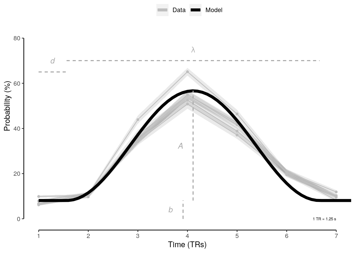
2.6.2.7 Source Data File Fig. 2c
dt_odd_long_mean %>%
select(-classification, -num_subs) %>%
write.csv(., file = file.path(path_sourcedata, "source_data_figure_2c.csv"),
row.names = FALSE)2.6.3 Response model and difference dynamics
# get the average horizontal shift of the first sine wave:
t_first = mean(dt_odd_long_fit$shift)
# calculate the shift of the second sine wave (shift + half a wavelength)
t_second = mean(dt_odd_long_fit$shift) + add_shift + 1/mean(dt_odd_long_fit$freq)
# calculate the time point of cross over between the two sine functions:
t_crossover = 0.5/mean(dt_odd_long_fit$freq) + mean(dt_odd_long_fit$shift) + add_shift/2
# create a vector of time steps:
time = seq(0, 8, 0.1)
max_prob = max(dt_odd_long_fit_shift$probability[dt_odd_long_fit_shift$event == "difference"], na.rm = TRUE)
t_max_diff = dt_odd_long_fit_shift$t[dt_odd_long_fit_shift$probability == max_prob & !is.na(dt_odd_long_fit_shift$probability)]
a = dt_odd_long_fit_shift$probability[dt_odd_long_fit_shift$t == t_max_diff & dt_odd_long_fit_shift$event == "first"]2.6.3.1 Figure 2d
# select colors used for plotting:
colors = c("darkgray", "darkgray", "black", "dodgerblue", "red", "black")
# plot sine wave difference illustration:
fig_b = ggplot(data = dt_odd_long_fit_shift, aes(
x = time, y = probability * 100, group = event, color = event)) +
# create rectangles to indicate the forward and backward phase:
annotate("rect", xmin = t_first, xmax = t_crossover, ymin = -80, ymax = 95,
alpha = 0.05, fill = "dodgerblue") +
annotate("rect", xmin = t_crossover, xmax = t_second, ymin = -80, ymax = 95,
alpha = 0.05, fill = "red") +
# plot the onset of the first event:
geom_vline(xintercept = t_first, color = "gray", linetype = "dashed") +
# plot the offset of the second event (d + lambda + s in manuscript text):
geom_vline(xintercept = t_second, color = "gray", linetype = "dashed") +
# plot the crossover (d + 0.5 * (lambda + s) in manuscript text)
geom_vline(xintercept = t_crossover, color = "gray", linetype = "dashed") +
# plot the horizontal line for the difference time course:
geom_hline(yintercept = -20, color = "gray") +
# plot the horizontal line for the cosine wave:
geom_hline(yintercept = -60, color = "gray") +
# plot the first and second event time courses:
geom_line(aes(x = t, linetype = fct_rev(event)), na.rm = TRUE) +
coord_capped_cart(left = "both", bottom = "both", ylim = c(-80, 85)) +
xlab("Time (in TRs)") + ylab("Probability (a.u.)") +
scale_colour_manual(name = "Serial event", values = colors) +
scale_linetype_manual(values = c(rep("solid", 3), "dashed", "solid")) +
scale_x_continuous(labels = c(label_fill(seq(1,7,1), mod = 1), rep("", 2)),
breaks = seq(0,8,1)) +
theme(axis.text.y = element_blank(), axis.ticks.y = element_line(colour = "white"),
axis.line.y = element_line(colour = "white")) +
theme(legend.position = "none") +
annotate("label", x = 0.5, y = 45, label = "~1^'st'~event",
color = "dodgerblue", parse = TRUE, size = 3) +
annotate("label", x = 0.5, y = 30, label = "~2^'nd'~event",
color = "red", parse = TRUE, size = 3) +
annotate("label", x = 0.5, y = -7, label = "Difference",
color = "black", size = 3) +
annotate("label", x = 0.5, y = -35, label = "Difference\n(no flattening)",
color = "darkgray", size = 3) +
# add annotation for forward period:
geom_segment(aes(x = t_first, xend = t_crossover, yend = 85, y = 85,
colour = "segment"), color = "dodgerblue") +
annotate("label", x = t_first + (t_crossover - t_first)/2, y = 85,
label = "Forward period",
color = "dodgerblue", fill = "white", hjust = 0.5) +
# add annotations for backward period:
geom_segment(aes(x = t_crossover, xend = t_second, y = 85, yend = 85,
colour = "segment"), color = "red") +
annotate("label", x = t_crossover + (t_second - t_crossover)/2, y = 85,
label = "Backward period",
color = "red", fill = "white", hjust = 0.5) +
# add annotation for early forward phase
geom_segment(aes(x = t_first, xend = t_first + (t_crossover - t_first)/2, yend = 70, y = 70,
colour = "segment"), color = "gray") +
annotate("label", x = (t_first + (t_crossover - t_first)/4),
y = 70, label = "early",
color = "gray", fill = "white", hjust = 0.5) +
# add annotation for late forward phase
geom_segment(aes(x = t_first + (t_crossover - t_first)/2, xend = t_crossover,
yend = 68, y = 68, colour = "segment"), color = "gray") +
annotate("label", x = (t_first + (t_crossover - t_first)/4 * 3),
y = 68, label = "late",
color = "gray", fill = "white", hjust = 0.5) +
# add annotation for early backward phase
geom_segment(aes(x = t_crossover, xend = t_crossover + (t_second - t_crossover)/2,
yend = 70, y = 70, colour = "segment"), color = "gray") +
annotate("label", x = (t_crossover + (t_second - t_crossover)/4),
y = 70, label = "early", color = "gray", fill = "white", hjust = 0.5) +
# add annotation for late backward phase
geom_segment(aes(x = t_crossover + (t_second - t_crossover)/2, xend = t_second,
yend = 68, y = 68, colour = "segment"), color = "gray") +
annotate("label", x = (t_crossover + (t_second - t_crossover)/4 * 3),
y = 68, label = "late", color = "gray", fill = "white", hjust = 0.5) +
# add annotation for delta:
geom_segment(aes(x = t_first + (t_crossover - t_first)/2,
xend = t_first + (t_crossover - t_first)/2 + add_shift,
y = 35 , yend = 35, colour = "segment"), color = "darkgray", linetype = "dotted") +
annotate("text", x = t_first + (t_crossover - t_first)/2 - 0.5 + add_shift / 2, y = 36,
label = "delta", color = "darkgray", hjust = 0.5, parse = TRUE) +
# add annotation for TRs:
annotate("text", x = 8, y = -80, label = "1 TR = 1.25 s",
hjust = 1, size = rel(2)) +
theme(axis.line.x = element_line(colour = "black"),
panel.grid.major = element_blank(),
panel.grid.minor = element_blank(),
panel.border = element_blank(),
panel.background = element_blank())
fig_b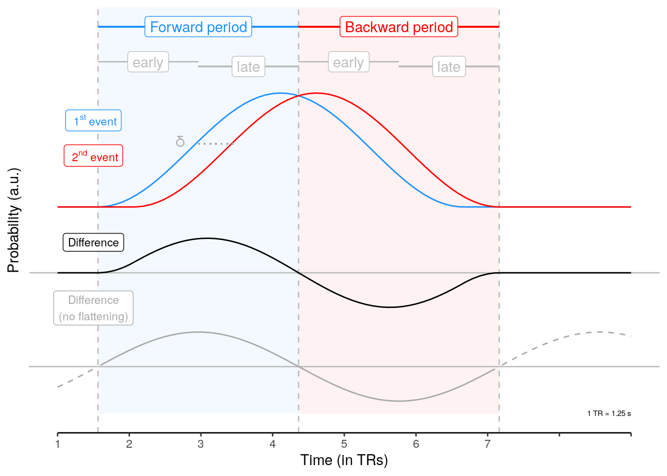
2.6.3.2 Source Data File Fig. 2d
dt_odd_long_fit_shift %>%
select(-classification) %>%
write.csv(., file = file.path(path_sourcedata, "source_data_figure_2d.csv"),
row.names = FALSE)ampfun = function(s, A) {A*cos(s*mean(dt_odd_long_fit$freq)*pi - 0.5*pi)}
cs = seq(0, 0.5/mean(dt_odd_long_fit$freq), 0.01)
ba = data.table(cs = cs, diff = ampfun(cs, 1))
fig_c = ggplot(data = ba, aes(x = cs, y = diff)) +
geom_line() +
xlab("Time-shift (in TRs)") + ylab("Max. diff. in amplitude") +
coord_capped_cart(left = "both", bottom = "both", xlim = c(0,3)) +
scale_x_continuous(labels = c("0", rep("", 2), "Resp. peak"), breaks = seq(0,3)) +
scale_y_continuous(labels = c("0", rep("", 3), "Max")) +
#theme(plot.margin = unit(c(t = 10, r = 30, b = 1, l = 1), "pt")) +
theme(axis.text.y = element_text(angle = 90, hjust = 0.5)) +
theme(axis.line = element_line(colour = "black"),
panel.grid.major = element_blank(),
panel.grid.minor = element_blank(),
panel.border = element_blank(),
panel.background = element_blank())
fig_c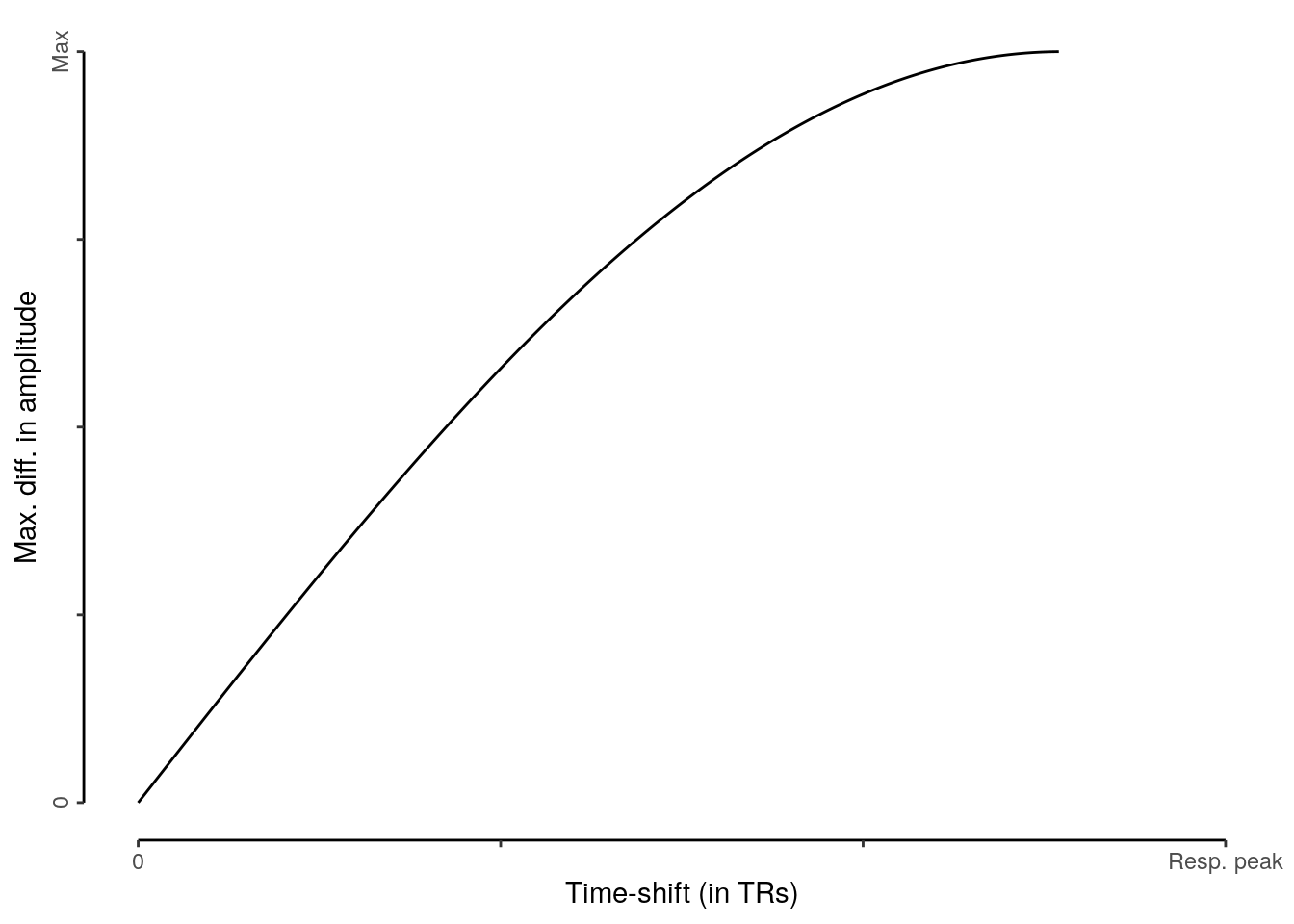
We plot a combination of the previous plots:
plot_grid(fig_a, fig_b, ncol = 2, hjust = c(0,0),
labels = c("c", "d", "e"), rel_widths = c(2, 4),
label_fontface = "bold", label_size = 14)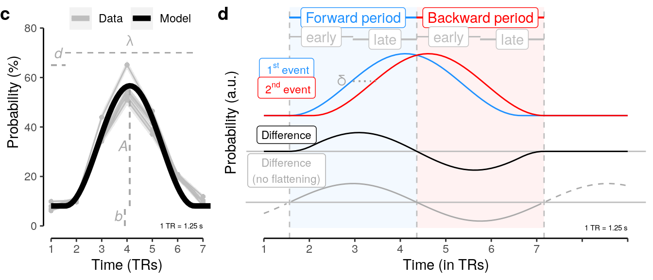
2.6.4 Forward and backward period for different speeds
Here, we calculate the expected forward and backward periods for two events separated by different speed levels (different values for delta).
calc_periods = function(speed, stim_dur = 0.1, num_stim = 5, tr = 1.25){
# mean wavelength based on fitted models, in TRs, round to two digits:
lambda = round(mean_parameters$mean_wavelength, 2)
# mean phase-shift based on fitted models, in TRs, round to two digits:
phase_shift = round(mean_parameters$mean_shift, 2)
# delta, in sec (time shift depending on speed)
delta_sec = stim_dur * (num_stim - 1) + (num_stim - 1) * speed
# delta, in trs:
delta_tr = delta_sec / tr
# end of forward period, in TRs:
fwd_end = 0.5 * (lambda + delta_tr) + phase_shift
# end of the backward period, in TRs:
bwd_end = lambda + phase_shift + delta_tr
# forward period, in TRs:
forward = list(seq(round(phase_shift) + 1, round(fwd_end - 0.5) + 1))
# backward period, in TRs:
backward = list(seq(round(fwd_end + 0.5) + 1, round(bwd_end) + 1))
# entire relevant trial period, in rounded TRs:
trial_period = list(seq(round(phase_shift) + 1, round(lambda + phase_shift + delta_tr) + 1))
# save results as a data table and return results:
dt = data.table(speed, lambda, delta_sec, delta_tr, fwd_end, bwd_end, forward, backward, trial_period)
return(dt)
}
# get the relevant timeperiods for each sequence speed condition:
speeds = c(0.032, 0.064, 0.128, 0.512, 2.048)
dt_periods = do.call(rbind, lapply(speeds, calc_periods))
rmarkdown::paged_table(dt_periods)We save the periods of interest for different speeds which will be used for the analysis of sequence and repetition trials:
save(dt_periods, file = file.path(path_root, 'data', "tmp", "dt_periods.Rdata"))2.6.5 Probability differences at different speeds
We plot the probability differences at different speeds:
time = seq(0, 12, 0.1)
speeds = c(0.032, 0.064, 0.128, 0.512, 2.048)
stim_dur = 0.1
dt_odd_seq_sim = dt_odd_long_fit %>% setDT(.) %>%
# average the fitted parameters across stimuli for each participant:
.[, by = .(classification, id), .(
mean_freq = mean(frequency),
mean_amplitude = mean(amplitude),
mean_shift = mean(shift),
mean_baseline = mean(baseline)
)] %>%
# repeat rows once for each speed condition (5 repetitions in total):
.[rep(seq(1, nrow(.)), length(speeds))] %>%
# add the different speed conditions for every participant:
.[, by = .(classification, id), ":=" (speed = speeds, num_events = 1)] %>%
# repeat rows once for each hypothetical event (here, 2 events):
.[rep(seq(1, nrow(.)), num_events)] %>%
# add a counter for the number of events:
.[, by = .(classification, id, speed), ":=" (event = 5)] %>%
# calculate a speed-specific shift for each event:
.[, by = .(classification, id, speed, event), {
shift = (speed * (event - 1) + (event - 1) * stim_dur)/1.25
amp = mean_amplitude * sin(shift * 0.5 * mean_freq * pi)
freq = (1/(1/mean_freq + shift))
c_d = amp * sin(2 * pi * time * freq - 2 * pi * freq * mean_shift)
# flatten the tails of the response function
cidx = time < mean_shift | time > (mean_shift + (1 / freq))
c_d[cidx] = 0
# save the response function:
list(time = time, probability = c_d)
}] %>%
filter(classification == "ovr") %>% setDT(.)
dt_odd_seq_sim_diff = dt_odd_seq_sim %>%
.[, by = .(classification, speed, time), .(
num_subs = .N,
mean_difference = mean(probability),
sem_upper = mean(probability) + (sd(probability)/sqrt(.N)),
sem_lower = mean(probability) - (sd(probability)/sqrt(.N))
)] %>% verify(all(num_subs == 36))save(dt_odd_seq_sim_diff, file = file.path(
path_root, "data", "tmp", "dt_odd_seq_sim_diff.Rdata"))
save(dt_odd_seq_sim, file = file.path(
path_root, "data", "tmp", "dt_odd_seq_sim.Rdata"))2.6.5.1 Figure 2e
fig_seq_sim_diff = ggplot(data = dt_odd_seq_sim_diff, mapping = aes(
x = time, y = as.numeric(mean_difference), color = as.factor(speed * 1000),
fill = as.factor(speed * 1000))) +
geom_hline(aes(yintercept = 0), linetype = "solid", color = "gray") +
geom_ribbon(aes(ymin = sem_lower, ymax = sem_upper), alpha = 0.5, color = NA) +
geom_line() +
theme(legend.position = "top", legend.direction = "horizontal",
legend.justification = "center", legend.margin = margin(0, 0, 0, 0),
legend.box.margin = margin(t = 0, r = 0, b = -5, l = 0)) +
xlab("Time from sequence onset (TRs)") + ylab("Probability difference") +
scale_colour_viridis(name = "Speed (ms)", discrete = TRUE, option = "cividis") +
scale_fill_viridis(name = "Speed (ms)", discrete = TRUE, option = "cividis") +
coord_capped_cart(left = "both", bottom = "both", expand = TRUE,
ylim = c(-0.4, 0.4), xlim = c(0, 12)) +
scale_x_continuous(labels = label_fill(seq(1, 13, 1), mod = 4), breaks = seq(0, 12, 1)) +
guides(color = guide_legend(nrow = 1)) +
geom_segment(aes(x = 0, xend = 0, y = 0.01, yend = 0.4),
arrow = arrow(length = unit(5, "pt")), color = "darkgray") +
geom_segment(aes(x = 0, xend = 0, y = -0.01, yend = -0.4),
arrow = arrow(length = unit(5, "pt")), color = "darkgray") +
annotate(geom = "text", x = 0.4, y = 0.2, label = "Forward order",
color = "darkgray", angle = 90, size = 3) +
annotate(geom = "text", x = 0.4, y = -0.2, label = "Backward order",
color = "darkgray", angle = 90, size = 3) +
annotate("text", x = 12, y = -0.4, label = "1 TR = 1.25 s",
hjust = 1, size = rel(2)) +
theme(axis.line = element_line(colour = "black"),
panel.grid.major = element_blank(),
panel.grid.minor = element_blank(),
panel.border = element_blank(),
panel.background = element_blank())
fig_seq_sim_diff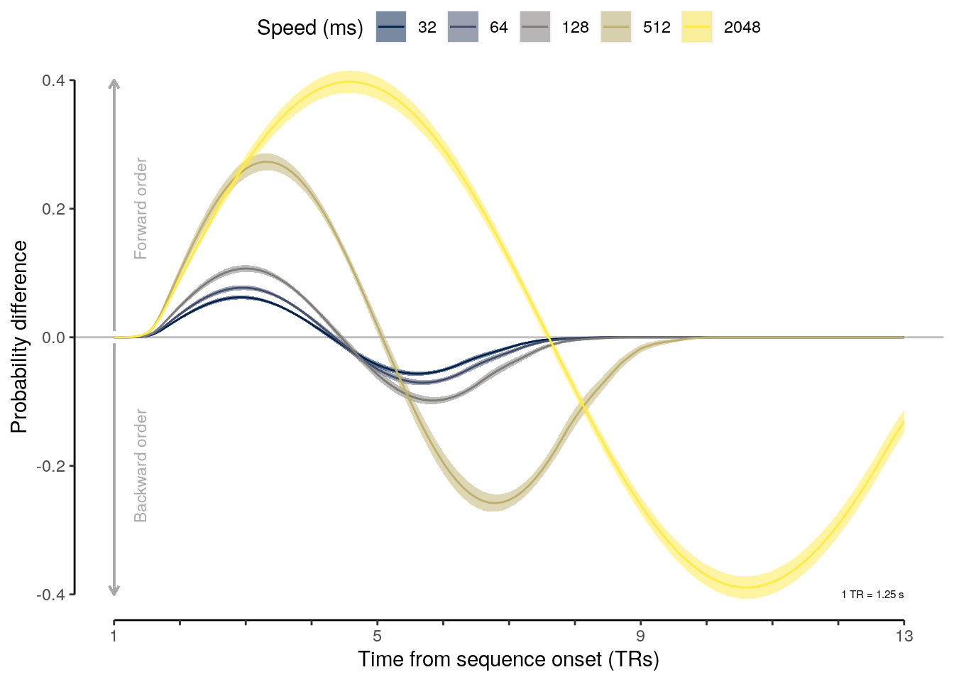
2.6.5.2 Source Data File Fig. 2e
dt_odd_seq_sim_diff %>%
select(-num_subs, -classification) %>%
write.csv(., file = file.path(path_sourcedata, "source_data_figure_2e.csv"),
row.names = FALSE)2.6.6 Figure 2
upper = plot_grid(fig_odd_peak, plot.odd.long, fig_a, labels = c("a", "b", "c"), ncol = 3,
rel_widths = c(0.8, 3.5, 2), label_fontface = "bold", hjust = c(0, 0))
lower = plot_grid(fig_b, fig_seq_sim_diff, labels = c("d", "e"), nrow = 1,
label_fontface = "bold", hjust = c(0, 0), rel_widths = c(0.45, 0.53))
plot_grid(upper, lower, nrow = 2, ncol = 1, rel_heights = c(2.5, 3))
ggsave(filename = "highspeed_plot_decoding_oddball_data.pdf",
plot = last_plot(), device = cairo_pdf, path = path_figures, scale = 1,
dpi = "retina", width = 10, height = 6.5)
ggsave(filename = "wittkuhn_schuck_figure_2.pdf",
plot = last_plot(), device = cairo_pdf, path = path_figures, scale = 1,
dpi = "retina", width = 10, height = 6.5)2.7 Decoding: Sequence trials
2.7.1 Initialization
2.7.1.1 Load data and files
We load the data and relevant functions:
# find the path to the root of this project:
if (!requireNamespace("here")) install.packages("here")
if ( basename(here::here()) == "highspeed" ) {
path_root = here::here("highspeed-analysis")
} else {
path_root = here::here()
}
# source all relevant functions from the setup R script:
load(file.path(path_root, "data", "tmp", "dt_periods.Rdata"))
load(file.path(path_root, "data", "tmp", "dt_odd_seq_sim_diff.Rdata"))
load(file.path(path_root, "data", "tmp", "dt_odd_seq_sim.Rdata"))
sub_exclude <- c("sub-24", "sub-31", "sub-37", "sub-40")The next step is only evaluated during manual execution:
# source all relevant functions from the setup R script:
source(file.path(path_root, "code", "highspeed-analysis-setup.R"))2.7.1.2 Data preparation
We create a function to determine early and late zones of forward and backward periods:
get_zones = function(trs_in){
if (length(trs_in) == 3) {
early = trs_in[c(2)]
late = trs_in[c(3)]
} else if (length(trs_in) == 4) {
early = trs_in[c(2)]
late = trs_in[c(4)]
} else if (length(trs_in) == 5) {
early = trs_in[c(2)]
late = trs_in[c(4)]
} else if (length(trs_in) == 6) {
early = trs_in[c(2, 3)]
late = trs_in[c(5, 6)]
} else if (length(trs_in) == 7) {
early = trs_in[c(2, 3)]
late = trs_in[c(5, 6)]
}
return(list(early = early, late = late))
}We prepare event and decoding data of sequence trials:
# create a subset of the events data table only including sequence task events:
dt_events_seq = dt_events %>%
filter(condition == "sequence" & trial_type == "stimulus")
# create a subset of the decoding data only including the sequence task data:
dt_pred_seq = dt_pred %>%
filter(condition == "sequence" & class != "other" & mask == "cv" & stim != "cue") %>%
setDT(.) %>%
# add serial position, change trial and target cue to the sequence data table:
.[, c("position", "change", "trial_cue", "accuracy", "trial_cue_position") := get_pos(
.SD, dt_events_seq), by = .(id, trial, class), .SDcols = c("id", "trial", "class")] %>%
# add variable to later pool trial_cue_position 1 to 3:
mutate(cue_pos_label = ifelse(trial_cue_position <= 3, "1-3", trial_cue_position)) %>%
setDT(.)We define the forward and backward periods depending on the response functions:
# define forward and backward period depending on response functions:
for (cspeed in unique(dt_pred_seq$tITI)) {
for (period in c("forward", "backward")) {
# get trs in the relevant forward or backward period based on response functions:
trs_period = dt_periods[[which(dt_periods$speed == cspeed), period]]
# set the period variable in the sequence data table accordingly:
dt_pred_seq$period[
dt_pred_seq$tITI %in% cspeed & dt_pred_seq$seq_tr %in% trs_period] = period
for (zone in c("early", "late")) {
trs_zone = get_zones(trs_period)[[zone]]
dt_pred_seq$zone[
dt_pred_seq$tITI %in% cspeed & dt_pred_seq$seq_tr %in% trs_zone] = zone
}
}
}
# assign the excluded label to all trs that are not in the forward or backward period:
dt_pred_seq$period[is.na(dt_pred_seq$period)] = "excluded"We exclude all participants with below-chance performance from the analyses:
# exclude participants with below-chance performance:
dt_pred_seq = dt_pred_seq %>%
filter(!(id %in% sub_exclude)) %>%
verify(length(unique(id)) == 36) %>%
setDT(.)We calculate the number of correct and incorrect sequence trials:
dt_num_correct <- dt_pred_seq %>%
# calculate the number of trials for each accuracy level for each participant:
.[, by = .(classification, id, accuracy), .(
num_trials = length(unique(trial))
)] %>%
# select only the one-versus-rest decoding approach:
filter(classification == "ovr") %>%
setDT(.) %>%
# verify that the sum of all trials equals 75 for all participants:
verify(.[, by = .(classification, id), .(
sum_trials = sum(num_trials))]$sum_trials == 75) %>%
# complete missing values for number of trials for each accuracy level:
complete(classification, id, accuracy, fill = list(num_trials = 0)) %>%
setDT(.) %>%
# verify that there are two accuracy levels per participant:
verify(.[, by = .(classification, id), .(
num_acc_levels = .N)]$num_acc_levels == 2) %>%
# calculate the mean number of (in)accurate trials per participant:
.[, by = .(classification, accuracy), .(
num_subs = .N,
mean_num_trials = mean(num_trials),
percent_trials = mean(num_trials)/75
)]
# print formatted table:
rmarkdown::paged_table(dt_num_correct)2.7.2 Probability time courses
We calculate the decoding probability time-courses:
# select the variable of interest:
variable = "probability_norm"
dt_pred_seq_prob = dt_pred_seq %>%
# average across trials separately for each position, TR, and participant
.[, by = .(id, classification, tITI, period, seq_tr, position), .(
num_trials = .N,
mean_prob = mean(get(variable)) * 100
)] %>%
# check if the averaged data consists of 15 sequence trial per participant:
verify(all(num_trials == 15)) %>%
# average across participants and calculate standard error of the mean:
.[, by = .(classification, tITI, period, seq_tr, position), .(
num_subs = .N,
mean_prob = mean(mean_prob),
sem_upper = mean(mean_prob) + (sd(mean_prob)/sqrt(.N)),
sem_lower = mean(mean_prob) - (sd(mean_prob)/sqrt(.N))
)] %>%
# check if averaged data is consistent with expected number of participants:
verify(all(num_subs == 36)) %>%
# create a new variable that expresses TRs as time from stimulus onset:
mutate(time = (seq_tr - 1) * 1.25) %>%
setDT(.)2.7.2.1 Figure 3a
We plot the decoding probability time-courses:
plot_raw_probas = function(dt1){
dt_reduced = dt1 %>%
setDT(.) %>%
.[, by = .(classification, tITI, period), .(
xmin = min(seq_tr) - 0.5,
xmax = max(seq_tr) + 0.5
)] %>%
filter(period != "excluded") %>%
mutate(fill = ifelse(period == "forward", "dodgerblue", "red"))
plot = ggplot(data = dt1, mapping = aes(
x = as.factor(seq_tr), y = as.numeric(mean_prob),
group = as.factor(position)), environment = environment()) +
geom_rect(data = dt_reduced, aes(
xmin = xmin, xmax = xmax, ymin = 0, ymax = 40),
alpha = 0.05, inherit.aes = FALSE, show.legend = FALSE, fill = dt_reduced$fill) +
facet_wrap(facets = ~ as.factor(tITI), labeller = get_labeller(array = dt1$tITI), nrow = 1) +
geom_ribbon(aes(ymin = sem_lower, ymax = sem_upper,
fill = as.factor(position)), alpha = 0.5) +
geom_line(mapping = aes(color = as.factor(position))) +
theme(legend.position = "top", legend.direction = "horizontal",
legend.justification = "center", legend.margin = margin(0, 0, 0, 0),
legend.box.margin = margin(t = 0, r = 0, b = -5, l = 0)) +
xlab("Time from sequence onset (TRs; 1 TR = 1.25 s)") +
ylab("Probability (%)") +
scale_color_manual(values = color_events, name = "Serial event") +
scale_fill_manual(values = color_events, name = "Serial event") +
scale_x_discrete(labels = label_fill(seq(1, 13, 1), mod = 4), breaks = seq(1, 13, 1)) +
coord_capped_cart(left = "both", bottom = "both", expand = TRUE, ylim = c(0, 25)) +
theme(panel.border = element_blank(), axis.line = element_line()) +
theme(axis.line = element_line(colour = "black"),
panel.grid.major = element_blank(),
panel.grid.minor = element_blank(),
panel.border = element_blank(),
panel.background = element_blank()) +
theme(strip.text.x = element_text(margin = margin(b = 2, t = 2))) +
guides(color = guide_legend(nrow = 1))
return(plot)
}
fig_seq_probas = plot_raw_probas(dt1 = subset(dt_pred_seq_prob, classification == "ovr"))
fig_seq_probas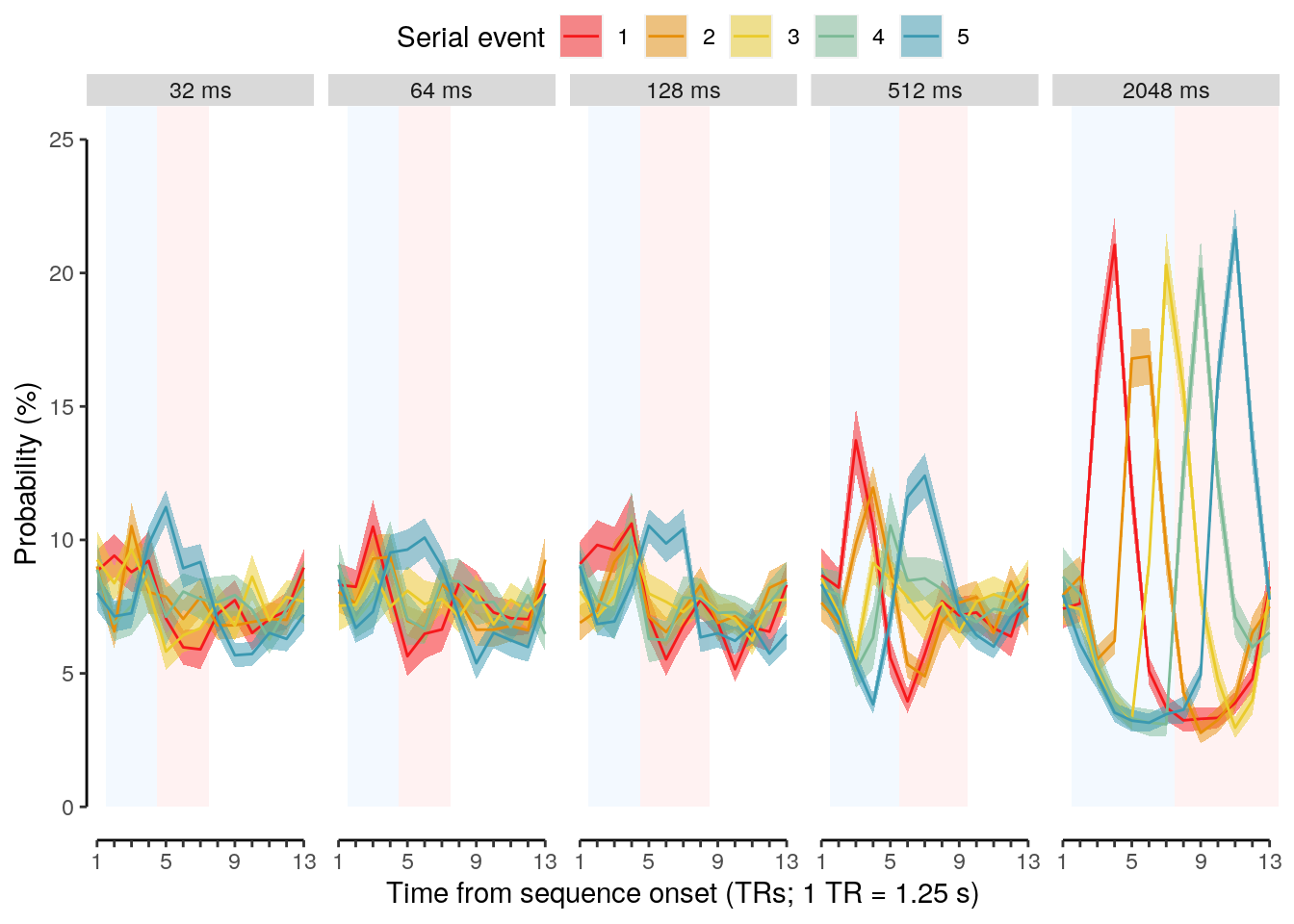
2.7.2.2 Source Data File Fig. 3a
subset(dt_pred_seq_prob, classification == "ovr") %>%
select(-classification, -num_subs) %>%
write.csv(., file = file.path(path_sourcedata, "source_data_figure_3a.csv"),
row.names = FALSE)We plot the decoding probabilities as a heat-map:
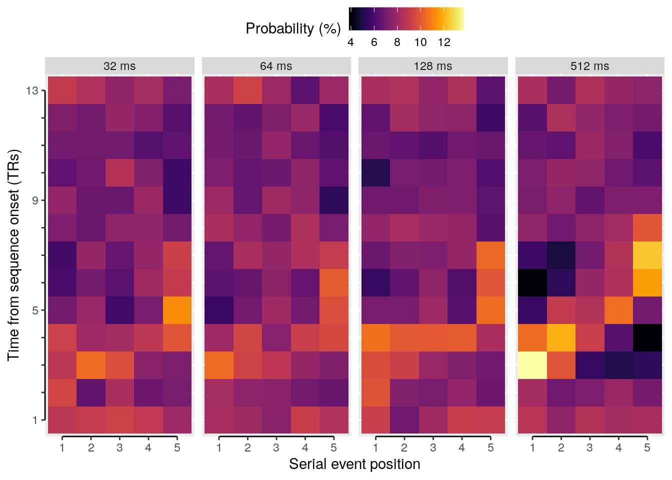
2.7.3 Influence of target cue position
We analyze the probabilities by target cue position:
# select the variable of interest:
variable = "probability_norm"
dt_pred_seq_prob_cue = dt_pred_seq %>%
# average across trials separately for each position, TR, and participant
.[, by = .(id, classification, tITI, period, seq_tr, position, cue_pos_label), .(
num_trials = .N,
mean_prob = mean(get(variable)) * 100
)] %>%
# average across participants and calculate standard error of the mean:
.[, by = .(classification, tITI, period, seq_tr, position,cue_pos_label), .(
num_subs = .N,
mean_num_trials = mean(num_trials),
sd_num_trials = sd(num_trials),
mean_prob = mean(mean_prob),
sem_upper = mean(mean_prob) + (sd(mean_prob)/sqrt(.N)),
sem_lower = mean(mean_prob) - (sd(mean_prob)/sqrt(.N))
)] %>%
# check if averaged data is consistent with expected number of participants:
verify(all(num_subs == 36)) %>%
# check that the SD of the number of trials per cue position is 0
# which means that each participant has the same number of trials per cue position:
verify(all(sd_num_trials == 0)) %>%
verify(all(mean_num_trials == 5)) %>%
# create a new variable that expresses TRs as time from stimulus onset:
mutate(time = (seq_tr - 1) * 1.25) %>%
transform(tITI = paste0(as.numeric(tITI) * 1000, " ms")) %>%
transform(tITI = factor(tITI, levels = c(
"32 ms", "64 ms", "128 ms", "512 ms", "2048 ms"))) %>%
setDT(.)We plot the probabilities by target cue position:
plot_raw_probas_cue = function(dt1){
plot = ggplot(data = dt1, mapping = aes(
x = as.factor(seq_tr), y = as.numeric(mean_prob),
group = as.factor(position))) +
facet_grid(rows = vars(cue_pos_label), cols = vars(tITI)) +
geom_ribbon(aes(ymin = sem_lower, ymax = sem_upper,
fill = as.factor(position)), alpha = 0.5) +
geom_line(mapping = aes(color = as.factor(position))) +
theme(legend.position = "top", legend.direction = "horizontal",
legend.justification = "center", legend.margin = margin(0, 0, 0, 0),
legend.box.margin = margin(t = 0, r = 0, b = -5, l = 0)) +
xlab("Time from sequence onset (TRs)") + ylab("Probability (%)") +
scale_color_manual(values = color_events, name = "Serial event") +
scale_fill_manual(values = color_events, name = "Serial event") +
scale_x_discrete(labels = label_fill(seq(1, 13, 1), mod = 4), breaks = seq(1, 13, 1)) +
coord_capped_cart(left = "both", bottom = "both", expand = TRUE, ylim = c(0, 25)) +
theme(panel.border = element_blank(), axis.line = element_line()) +
theme(axis.line = element_line(colour = "black"),
panel.grid.major = element_blank(),
panel.grid.minor = element_blank(),
panel.border = element_blank(),
panel.background = element_blank())
theme(strip.text.x = element_text(margin = margin(b = 2, t = 2))) +
guides(color = guide_legend(nrow = 1))
return(plot)
}
fig_seq_probas_cue = plot_raw_probas_cue(dt1 = subset(dt_pred_seq_prob_cue, classification == "ovr"))
fig_seq_probas_cue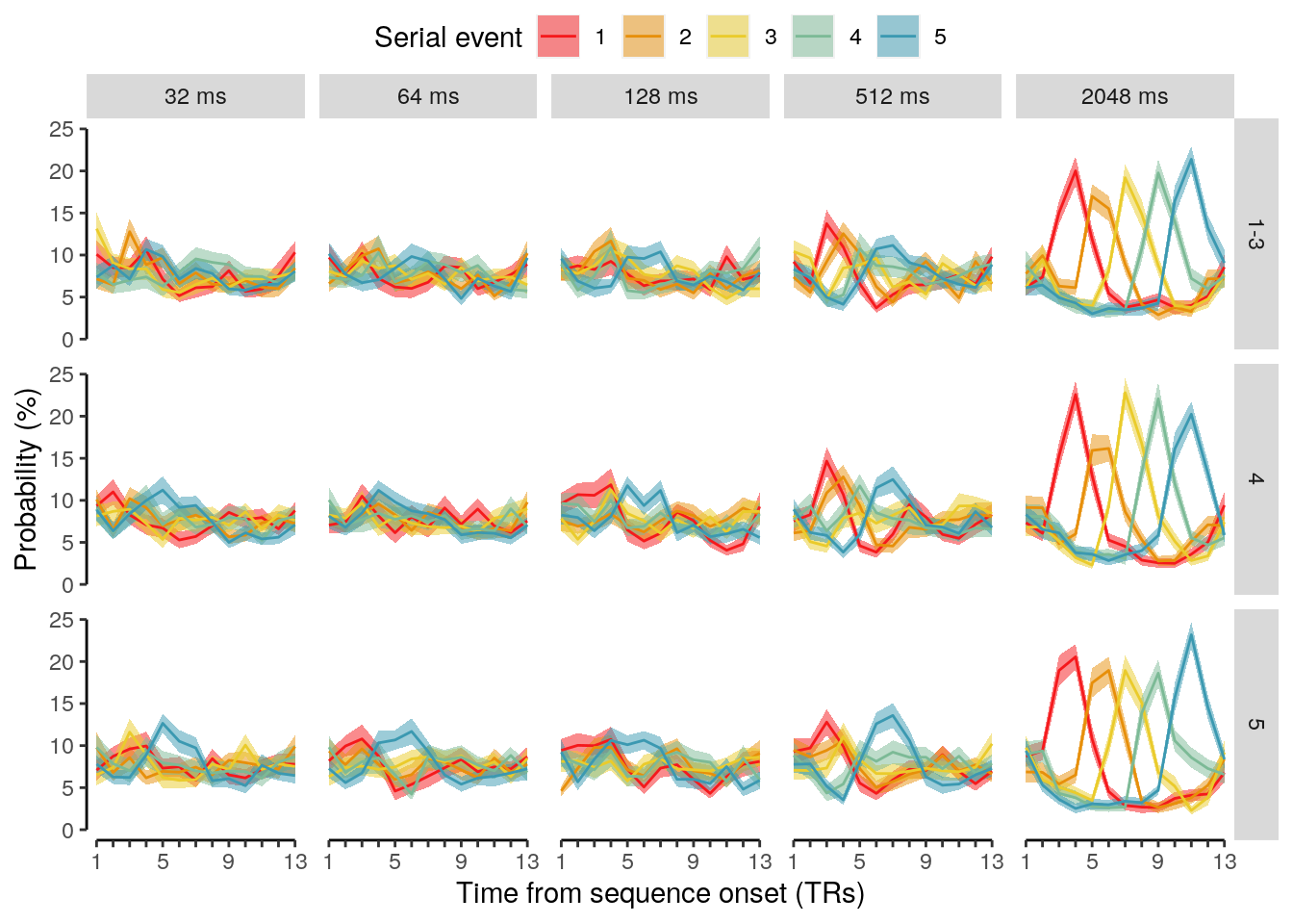
2.7.4 Regression slope timecourses
We compare the mean indices of association (regression slope, correlation, mean serial position) for every TR:
# select positions within every TR that should be selected:
pos_sel = seq(1, 5)
# define relevant variables:
variable = "probability_norm"
cor_method = "kendall"
# calculate indices of association at every TR:
dt_pred_seq_cor = dt_pred_seq %>%
# here, we can filter for specific sequence events:
filter(position %in% seq(1, 5, by = 1)) %>%
setDT(.) %>%
# order positions by decreasing probability and calculate step size
# calculate correlation and slope between position and probability
# verify that there are five probabilities (one for each class) per volume
# verify that all correlations range between -1 and 1
.[, by = .(id, classification, tITI, period, trial_tITI, seq_tr), {
# order the probabilities in decreasing order (first = highest):
prob_order_idx = order(get(variable), decreasing = TRUE)
# order the positions by probability:
pos_order = position[prob_order_idx]
# order the probabilities:
prob_order = get(variable)[prob_order_idx]
# select positions
pos_order_sel = pos_order[pos_sel]
prob_order_sel = prob_order[pos_sel]
list(
# calculate the number of events:
num_events = length(pos_order_sel[!is.na(pos_order_sel)]),
# calculate the mean step size between probability-ordered events:
mean_step = mean(diff(pos_order_sel)),
# calculate the mean correlation between positions and their probabilities:
cor = cor.test(pos_order_sel, prob_order_sel, method = cor_method)$estimate,
# calculate the slope of a linear regression between position and probabilities:
slope = coef(lm(prob_order_sel ~ pos_order_sel))[2]
# verify that the number of events matches selection and correlations -1 < r < 1
)}] %>% verify(all(num_events == length(pos_sel))) %>% #verify(between(cor, -1, 1)) %>%
# average across trials for each participant (flip values by multiplying with -1):
# verify that the number of trials per participant is correct:
.[, by = .(id, classification, tITI, period, seq_tr), .(
num_trials = .N,
mean_cor = mean(cor) * (-1),
mean_step = mean(mean_step),
mean_slope = mean(slope) * (-1)
)] %>%
verify(all(num_trials == 15)) %>%
# shorten the period name:
mutate(period_short = ifelse(period == "forward", "fwd", period)) %>%
transform(period_short = ifelse(period == "backward", "bwd", period_short)) %>%
mutate(color = ifelse(period_short == "fwd", "dodgerblue", "red")) %>% setDT(.)We compare the mean indices of association (regression slope, correlation, mean serial position) against zero (the expectation of no association) for every TR:
seq_test_time <- function(data, variable){
data_out = data %>%
# average across participants for every speed at every TR:
# check if the number of participants matches:
.[, by = .(classification, tITI, period, seq_tr), {
# perform a two-sided one-sample t-test against zero (baseline):
ttest_results = t.test(get(variable), alternative = "two.sided", mu = 0);
list(
num_subs = .N,
mean_variable = mean(get(variable)),
pvalue = ttest_results$p.value,
tvalue = ttest_results$statistic,
df = ttest_results$parameter,
cohens_d = round(abs(mean(mean(get(variable)) - 0)/sd(get(variable))), 2),
sem_upper = mean(get(variable)) + (sd(get(variable))/sqrt(.N)),
sem_lower = mean(get(variable)) - (sd(get(variable))/sqrt(.N))
)}] %>% verify(all(num_subs == 36)) %>% verify(all((num_subs - df) == 1)) %>%
# adjust p-values for multiple comparisons (filter for forward and backward period):
# check if the number of comparisons matches expectations:
.[period %in% c("forward", "backward"), by = .(classification), ":=" (
num_comp = .N,
pvalue_adjust = p.adjust(pvalue, method = "fdr", n = .N)
)] %>% verify(all(num_comp == 39, na.rm = TRUE)) %>%
# round the original p-values according to the apa standard:
mutate(pvalue_round = round_pvalues(pvalue)) %>%
# round the adjusted p-value:
mutate(pvalue_adjust_round = round_pvalues(pvalue_adjust)) %>%
# sort data table:
setorder(., classification, period, tITI, seq_tr) %>%
# create new variable indicating significance below 0.05
mutate(significance = ifelse(pvalue_adjust < 0.05, "*", ""))
return(data_out)
}# filter for significant p-values to make reporting easier:
rmarkdown::paged_table(seq_test_time(data = dt_pred_seq_cor, variable = "mean_cor") %>%
filter(pvalue_adjust < 0.05, classification == "ovr"))rmarkdown::paged_table(seq_test_time(data = dt_pred_seq_cor, variable = "mean_step") %>%
filter(pvalue_adjust < 0.05, classification == "ovr"))rmarkdown::paged_table(seq_test_time(data = dt_pred_seq_cor, variable = "mean_slope") %>%
filter(pvalue_adjust < 0.05, classification == "ovr"))plot_seq_cor_time = function(dt, variable){
# select the variable of interest, determine y-axis label and adjust axis:
if (variable == "mean_slope") {
ylabel = "Regression slope"
adjust_axis = 0.1
} else if (variable == "mean_cor") {
ylabel = expression("Correlation ("*tau*")")
adjust_axis = 1
} else if (variable == "mean_step") {
ylabel = "Mean step size"
adjust_axis = 1
}
plot = ggplot(data = dt, mapping = aes(
x = seq_tr, y = mean_variable, group = as.factor(as.numeric(tITI) * 1000),
fill = as.factor(as.numeric(tITI) * 1000))) +
geom_hline(aes(yintercept = 0), linetype = "solid", color = "gray") +
geom_ribbon(aes(ymin = sem_lower, ymax = sem_upper), alpha = 0.5, color = NA) +
geom_line(mapping = aes(color = as.factor(as.numeric(tITI) * 1000))) +
xlab("Time from sequence onset (TRs)") + ylab(ylabel) +
scale_colour_viridis(name = "Speed (ms)", discrete = TRUE, option = "cividis") +
scale_fill_viridis(name = "Speed (ms)", discrete = TRUE, option = "cividis") +
scale_x_continuous(labels = label_fill(seq(1, 13, 1), mod = 4), breaks = seq(1, 13, 1)) +
guides(color = guide_legend(nrow = 1)) +
annotate("text", x = 1, y = -0.4 * adjust_axis, label = "1 TR = 1.25 s",
hjust = 0, size = rel(2)) +
coord_capped_cart(left = "both", bottom = "both", expand = TRUE,
ylim = c(-0.4 * adjust_axis, 0.4 * adjust_axis)) +
theme(panel.border = element_blank(), axis.line = element_line()) +
theme(axis.line = element_line(colour = "black"),
panel.grid.major = element_blank(),
panel.grid.minor = element_blank(),
panel.border = element_blank(),
panel.background = element_blank()) +
theme(legend.position = "top", legend.direction = "horizontal",
legend.justification = "center", legend.margin = margin(t = 0, r = 0, b = 0, l = 0),
legend.box.margin = margin(t = 0, r = 0, b = 0, l = 0)) +
geom_segment(aes(x = 0.05, xend = 0.05, y = 0.01 * adjust_axis, yend = 0.4 * adjust_axis),
arrow = arrow(length = unit(5, "pt")), color = "darkgray") +
geom_segment(aes(x = 0.05, xend = 0.05, y = -0.01 * adjust_axis, yend = -0.4 * adjust_axis),
arrow = arrow(length = unit(5, "pt")), color = "darkgray") +
annotate(geom = "text", x = 0.4, y = 0.2 * adjust_axis, label = "Forward order",
color = "darkgray", angle = 90, size = 3) +
annotate(geom = "text", x = 0.4, y = -0.2 * adjust_axis, label = "Backward order",
color = "darkgray", angle = 90, size = 3)
return(plot)
}2.7.4.1 Figure 3b
fig_seq_cor_time = plot_seq_cor_time(dt = subset(
seq_test_time(data = dt_pred_seq_cor, variable = "mean_cor"),
classification == "ovr"), variable = "mean_cor")
fig_seq_slope_time = plot_seq_cor_time(dt = subset(
seq_test_time(data = dt_pred_seq_cor, variable = "mean_slope"),
classification == "ovr"), variable = "mean_slope")
fig_seq_step_time = plot_seq_cor_time(dt = subset(
seq_test_time(data = dt_pred_seq_cor, variable = "mean_step"),
classification == "ovr"), variable = "mean_step")
fig_seq_cor_time; fig_seq_slope_time; fig_seq_step_time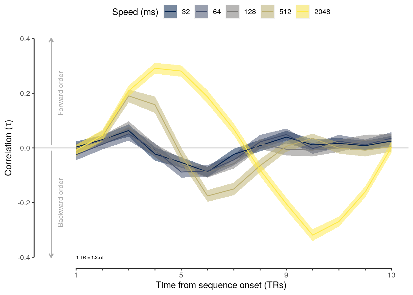
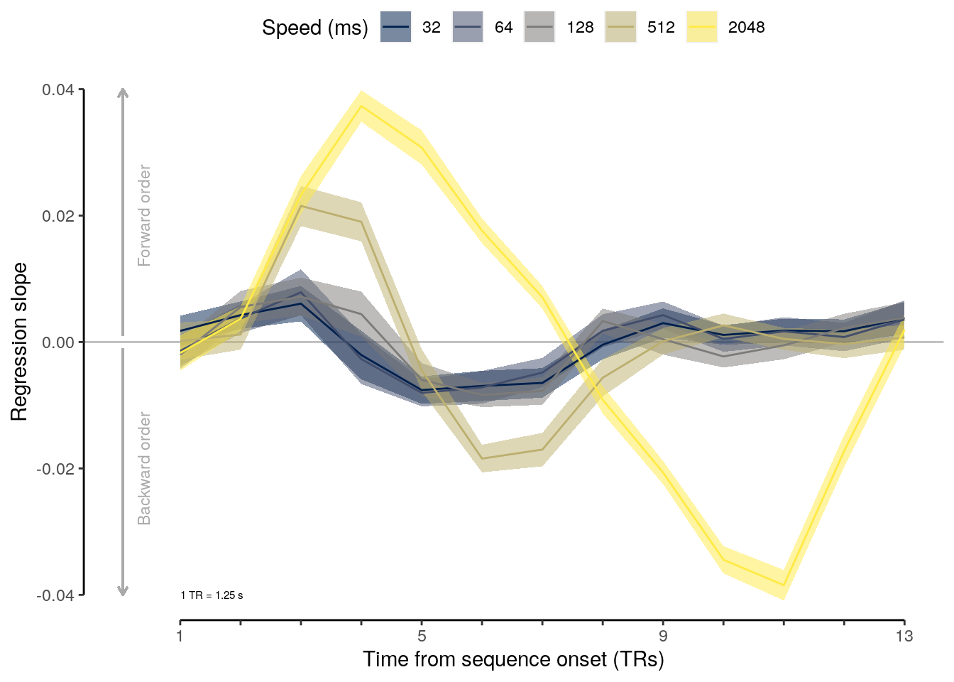
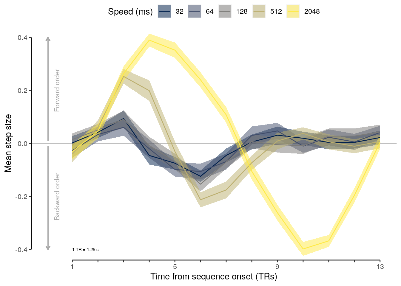
2.7.4.2 Source Data File Fig. 3b
subset(
seq_test_time(data = dt_pred_seq_cor, variable = "mean_slope"),
classification == "ovr") %>%
select(-classification, -num_subs, -num_comp, -pvalue_adjust,
-pvalue_round, -pvalue_adjust_round, -pvalue, -df, -cohens_d,
-tvalue, -significance) %>%
write.csv(., file = file.path(path_sourcedata, "source_data_figure_3b.csv"),
row.names = FALSE)2.7.4.3 Source Data File Fig. S5a
subset(
seq_test_time(data = dt_pred_seq_cor, variable = "mean_cor"),
classification == "ovr") %>%
select(-classification, -num_subs, -num_comp, -pvalue_adjust,
-pvalue_round, -pvalue_adjust_round, -pvalue, -df, -cohens_d,
-tvalue, -significance) %>%
write.csv(., file = file.path(path_sourcedata, "source_data_figure_s5a.csv"),
row.names = FALSE)2.7.4.4 Source Data File Fig. S5c
subset(
seq_test_time(data = dt_pred_seq_cor, variable = "mean_step"),
classification == "ovr") %>%
select(-classification, -num_subs, -num_comp, -pvalue_adjust,
-pvalue_round, -pvalue_adjust_round, -pvalue, -df, -cohens_d,
-tvalue, -significance) %>%
write.csv(., file = file.path(path_sourcedata, "source_data_figure_s5c.csv"),
row.names = FALSE)We test depending on the target cue position:
# select positions within every TR that should be selected:
pos_sel = seq(1, 5)
# define relevant variables:
variable = "probability_norm"
cor_method = "kendall"
# calculate indices of association at every TR:
dt_pred_seq_cor_cue = dt_pred_seq %>%
# here, we can filter for specific sequence events:
filter(position %in% seq(1, 5, by = 1)) %>% setDT(.) %>%
# order positions by decreasing probability and calculate step size
# calculate correlation and slope between position and probability
# verify that there are five probabilities (one for each class) per volume
# verify that all correlations range between -1 and 1
.[, by = .(id, classification, tITI, period, trial_tITI, seq_tr, cue_pos_label), {
# order the probabilities in decreasing order (first = highest):
prob_order_idx = order(get(variable), decreasing = TRUE)
# order the positions by probability:
pos_order = position[prob_order_idx]
# order the probabilities:
prob_order = get(variable)[prob_order_idx]
# select positions
pos_order_sel = pos_order[pos_sel]
prob_order_sel = prob_order[pos_sel]
list(
# calculate the number of events:
num_events = length(pos_order_sel[!is.na(pos_order_sel)]),
# calculate the mean step size between probability-ordered events:
mean_step = mean(diff(pos_order_sel)),
# calculate the mean correlation between positions and their probabilities:
cor = cor.test(pos_order_sel, prob_order_sel, method = cor_method)$estimate,
# calculate the slope of a linear regression between position and probabilities:
slope = coef(lm(prob_order_sel ~ pos_order_sel))[2]
# verify that the number of events matches selection and correlations -1 < r < 1
)}] %>% verify(all(num_events == length(pos_sel))) %>% #verify(between(cor, -1, 1)) %>%
# average across trials for each participant (flip values by multiplying with -1):
# verify that the number of trials per participant is correct:
.[, by = .(id, classification, tITI, period, seq_tr, cue_pos_label), .(
num_trials = .N,
mean_cor = mean(cor) * (-1),
mean_step = mean(mean_step),
mean_slope = mean(slope) * (-1)
)] %>%
verify(all(num_trials == 5)) %>%
# shorten the period name:
mutate(period_short = ifelse(period == "forward", "fwd", period)) %>%
transform(period_short = ifelse(period == "backward", "bwd", period_short)) %>%
mutate(color = ifelse(period_short == "fwd", "dodgerblue", "red")) %>% setDT(.)seq_test_time_cue <- function(data, variable){
data_out = data %>%
# average across participants for every speed at every TR:
# check if the number of participants matches:
.[, by = .(classification, tITI, period, seq_tr, cue_pos_label), {
# perform a two-sided one-sample t-test against zero (baseline):
ttest_results = t.test(get(variable), alternative = "two.sided", mu = 0);
list(
num_subs = .N,
mean_variable = mean(get(variable)),
pvalue = ttest_results$p.value,
tvalue = ttest_results$statistic,
df = ttest_results$parameter,
cohens_d = round(abs(mean(mean(get(variable)) - 0)/sd(get(variable))), 2),
sem_upper = mean(get(variable)) + (sd(get(variable))/sqrt(.N)),
sem_lower = mean(get(variable)) - (sd(get(variable))/sqrt(.N))
)}] %>% verify(all(num_subs == 36)) %>% verify(all((num_subs - df) == 1)) %>%
# adjust p-values for multiple comparisons (filter for forward and backward period):
# check if the number of comparisons matches expectations:
.[period %in% c("forward", "backward"), by = .(classification), ":=" (
num_comp = .N,
pvalue_adjust = p.adjust(pvalue, method = "fdr", n = .N)
)] %>% #verify(all(num_comp == 39, na.rm = TRUE)) %>%
# round the original p-values according to the apa standard:
mutate(pvalue_round = round_pvalues(pvalue)) %>%
# round the adjusted p-value:
mutate(pvalue_adjust_round = round_pvalues(pvalue_adjust)) %>%
# sort data table:
setorder(., classification, period, tITI, seq_tr) %>%
# create new variable indicating significance below 0.05
mutate(significance = ifelse(pvalue_adjust < 0.05, "*", ""))
return(data_out)
}fig_seq_slope_time_cue = plot_seq_cor_time_cue(dt = subset(
seq_test_time_cue(data = dt_pred_seq_cor_cue, variable = "mean_slope"),
classification == "ovr"), variable = "mean_slope")
fig_seq_slope_time_cue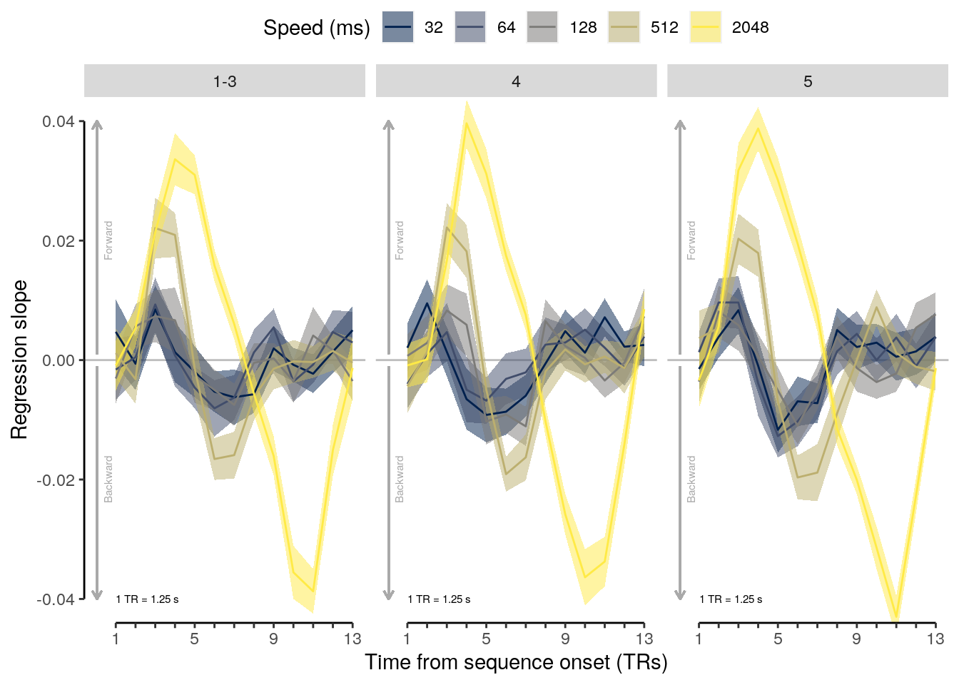
2.7.5 Correlation of regression time courses
2.7.5.1 Correlation between participants
We calculate the correlations between the predicted and the observed time courses between participants for each of the five speed conditions (inter-stimulus intervals):
# observed time courses:
dt_data_between = seq_test_time(
data = dt_pred_seq_cor, variable = "mean_slope") %>%
filter(classification == "ovr") %>%
transform(tITI = as.factor(as.numeric(tITI) * 1000)) %>%
setorder(classification, tITI, seq_tr)
# predicted time courses:
dt_model_between = dt_odd_seq_sim_diff %>%
transform(time = time + 1) %>%
filter(time %in% seq(1, 13, 1)) %>%
setorder(classification, speed, time)
# combine in one data table:
dt_between = data.table(
speed = dt_data_between$tITI,
tr = dt_data_between$seq_tr,
empirical = dt_data_between$mean_variable,
prediction = dt_model_between$mean_difference)
# calculate the correlation between
dt_between_results = dt_between %>%
.[, by = .(speed), {
cor = cor.test(empirical, prediction, method = "pearson")
list(
num_trs = .N,
pvalue = cor$p.value,
pvalue_round = round_pvalues(cor$p.value),
correlation = round(cor$estimate, 2)
)
}] %>%
verify(num_trs == 13) %>%
select(-num_trs)
# show the table with the correlations:
rmarkdown::paged_table(dt_between_results)2.7.5.2 Figure 3d
We plot the correlations between the regression slope time courses predicted by the model vs. the observed data between participants:
fig_seq_cor_between = ggplot(
data = dt_between,
mapping = aes(
x = prediction, y = empirical, color = speed, fill = speed)) +
geom_point(alpha = 1) +
geom_smooth(method = lm, se = FALSE, alpha = 0.5, fullrange = TRUE) +
scale_colour_viridis(
name = "Speed (ms)", discrete = TRUE,
option = "cividis", guide = FALSE) +
scale_fill_viridis(
name = "Speed (ms)", discrete = TRUE,
option = "cividis", guide = FALSE) +
xlab("Predicted slope") +
ylab("Observed slope") +
# guides(color = guide_legend(nrow = 1)) +
coord_capped_cart(
left = "both", bottom = "both", expand = TRUE,
xlim = c(-0.4, 0.4), ylim = c(-0.05, 0.05)) +
theme(legend.position = "top",
legend.direction = "horizontal",
legend.justification = "center",
legend.margin = margin(t = 0, r = 0, b = 0, l = 0),
legend.box.margin = margin(t = 0, r = 0, b = 0, l = 0)) +
theme(axis.line = element_line(colour = "black"),
panel.grid.major = element_blank(),
panel.grid.minor = element_blank(),
panel.border = element_blank(),
panel.background = element_blank())
# show the plot:
fig_seq_cor_between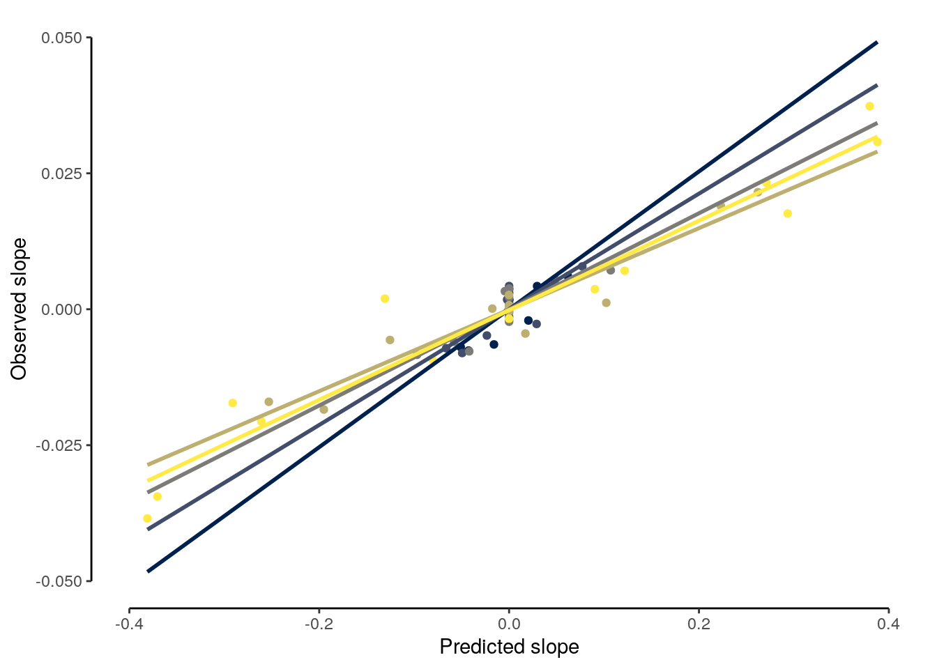
2.7.5.3 Source Data File Fig. 3d
dt_between %>%
write.csv(., file = file.path(path_sourcedata, "source_data_figure_3d.csv"),
row.names = FALSE)2.7.5.4 Correlation within participants
We calculate the correlations between the predicted and the observed time courses within participants for each of the five speed conditions (inter-stimulus intervals):
# observed regression slope time courses
dt_data_within = dt_pred_seq_cor %>%
filter(classification == "ovr") %>%
transform(tITI = as.factor(as.numeric(tITI) * 1000)) %>%
setorder(classification, id, tITI, seq_tr)
# predicted regression slope time courses
dt_model_within = dt_odd_seq_sim %>%
transform(time = time + 1) %>%
filter(time %in% seq(1, 13, 1)) %>%
setorder(classification, id, speed, time)
# combine in one data table:
dt_within = data.table(
id = dt_data_within$id,
speed = dt_data_within$tITI,
time = dt_data_within$seq_tr,
empirical = dt_data_within$mean_slope,
prediction = dt_model_within$probability)
# run correlations:
dt_within_cor = dt_within %>%
.[, by = .(id, speed), {
cor = cor.test(empirical, prediction, method = "pearson")
list(
num_trs = .N,
pvalue = cor$p.value,
estimate = as.numeric(cor$estimate)
)}] %>%
verify(num_trs == 13)
# run t-tests over correlation coefficients for each speed level:
dt_within_cor_results = setDT(dt_within_cor) %>%
.[, by = .(speed), {
ttest_results = t.test(
estimate, mu = 0, alternative = "two.sided", paired = FALSE)
list(
num_subs = .N,
mean_estimate = round(mean(estimate), 2),
pvalue = ttest_results$p.value,
tvalue = round(ttest_results$statistic, 2),
df = ttest_results$parameter,
cohens_d = round((mean(estimate) - 0)/sd(estimate), 2)
)}] %>%
verify(num_subs == 36) %>%
verify((num_subs - df) == 1) %>%
# adjust p-values for multiple comparisons:
# check if the number of comparisons matches expectations:
.[, ":=" (
num_comp = .N,
pvalue_adjust = p.adjust(pvalue, method = "fdr", n = .N)
)] %>%
# round the original p-values according to the apa standard:
mutate(pvalue_round = round_pvalues(pvalue)) %>%
# round the adjusted p-value:
mutate(pvalue_adjust_round = round_pvalues(pvalue_adjust)) %>%
# create new variable indicating significance below 0.05
mutate(significance = ifelse(pvalue_adjust < 0.05, "*", ""))
# show the table with the t-test results:
rmarkdown::paged_table(dt_within_cor_results)2.7.5.5 Figure 3e
We plot the correlations between the predicted and the observed time courses within participants for each of the five speed conditions (inter-stimulus intervals):
fig_seq_cor_within = ggplot(
data = dt_within_cor,
mapping = aes(
x = speed, y = estimate, color = speed, fill = speed, group = speed)) +
stat_summary(geom = "bar", fun = "mean") +
geom_dotplot(binaxis = "y", stackdir = "center", stackratio = 0.5,
color = "white", alpha = 0.5,
inherit.aes = TRUE, binwidth = 0.05) +
stat_summary(geom = "errorbar", fun.data = "mean_se", width = 0, color = "black") +
scale_colour_viridis(
name = "Speed (ms)", discrete = TRUE, option = "cividis", guide = FALSE) +
scale_fill_viridis(
name = "Speed (ms)", discrete = TRUE, option = "cividis", guide = FALSE) +
xlab("Speed (in ms)") +
ylab("Correlation (r)") +
#guides(color = guide_legend(nrow = 1)) +
coord_capped_cart(left = "both", bottom = "both", expand = TRUE) +
theme(legend.position = "top", legend.direction = "horizontal",
legend.justification = "center", legend.margin = margin(t = 0, r = 0, b = 0, l = 0),
legend.box.margin = margin(t = 0, r = 0, b = 0, l = 0)) +
theme(axis.ticks.x = element_line(colour = "white"),
axis.line.x = element_line(colour = "white")) +
theme(axis.title.x = element_blank(), axis.text.x = element_blank()) +
theme(axis.line = element_line(colour = "black"),
panel.grid.major = element_blank(),
panel.grid.minor = element_blank(),
panel.border = element_blank(),
panel.background = element_blank())
# show figure:
fig_seq_cor_within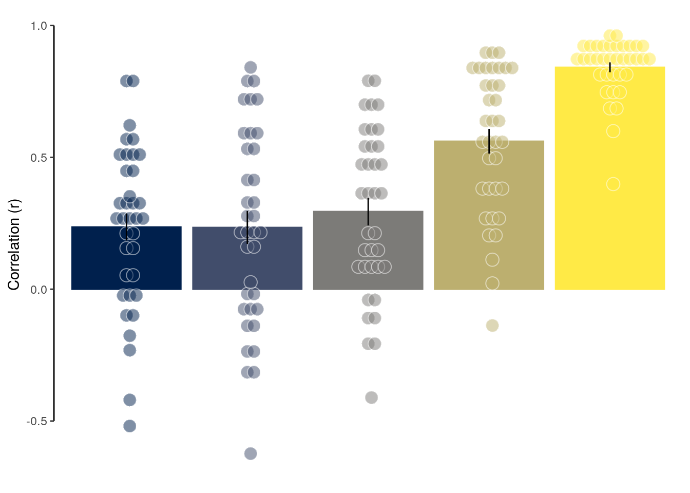
2.7.5.6 Source Data File Fig. 3e
dt_within_cor %>%
select(-num_trs, -pvalue) %>%
write.csv(., file = file.path(path_sourcedata, "source_data_figure_3e.csv"),
row.names = FALSE)2.7.6 Regression slope means
Calculate the average correlation or average regression slope for each time period (forward versus backward) for all five speed conditions:
seq_test_period <- function(data, variable){
data_out = data %>%
# filter out the excluded time period (select only forward and backward period):
filter(period != "excluded") %>%
setDT(.) %>%
# average for each time period and speed condition for every participant:
.[, by = .(classification, id, tITI, period), .(
mean_variable = mean(get(variable)))] %>%
# average across participants for every speed at every TR:
# check if the number of participants matches:
.[, by = .(classification, tITI, period), {
# perform a two-sided one-sample t-test against zero (baseline):
ttest_results = t.test(mean_variable, alternative = "two.sided", mu = 0);
list(
num_subs = .N,
mean_variable = mean(mean_variable),
pvalue = ttest_results$p.value,
tvalue = round(abs(ttest_results$statistic), 2),
df = ttest_results$parameter,
cohens_d = abs(round((mean(mean_variable) - 0) / sd(mean_variable), 2)),
sem_upper = mean(mean_variable) + (sd(mean_variable)/sqrt(.N)),
sem_lower = mean(mean_variable) - (sd(mean_variable)/sqrt(.N))
)
}] %>%
verify(all(num_subs == 36)) %>%
verify(all((num_subs - df) == 1)) %>%
# adjust p-values for multiple comparisons:
# check if the number of comparisons matches expectations:
.[period %in% c("forward", "backward"), by = .(classification), ":=" (
num_comp = .N,
pvalue_adjust = p.adjust(pvalue, method = "fdr", n = .N)
)] %>%
verify(num_comp == 10) %>%
# add variable that indicates significance with stupid significance stars:
mutate(significance = ifelse(pvalue < 0.05, "*", "")) %>%
# round the original p-values according to APA manual:
mutate(pvalue_round = round_pvalues(pvalue)) %>%
# round the adjusted p-value:
mutate(pvalue_adjust_round = round_pvalues(pvalue_adjust)) %>%
# sort data table:
setorder(classification, period, tITI) %>%
# shorten the period name:
mutate(period_short = ifelse(period == "forward", "fwd", period)) %>%
transform(period_short = ifelse(period == "backward", "bwd", period_short)) %>%
mutate(color = ifelse(period_short == "fwd", "dodgerblue", "red")) %>% setDT(.)
return(data_out)
}rmarkdown::paged_table(
seq_test_period(data = dt_pred_seq_cor, variable = "mean_cor") %>%
filter(pvalue_adjust < 0.05, classification == "ovr"))rmarkdown::paged_table(
seq_test_period(data = dt_pred_seq_cor, variable = "mean_step") %>%
filter(pvalue_adjust < 0.05, classification == "ovr"))rmarkdown::paged_table(
seq_test_period(data = dt_pred_seq_cor, variable = "mean_slope") %>%
filter(pvalue_adjust < 0.05, classification == "ovr"))2.7.6.1 Figure 3c
plot_seq_cor_period = function(data, variable){
# select the variable of interest, determine y-axis label and adjust axis:
if (variable == "mean_slope") {
ylabel = "Regression slope"
adjust_axis = 0.1
} else if (variable == "mean_cor") {
ylabel = expression("Correlation ("*tau*")")
adjust_axis = 1
} else if (variable == "mean_step") {
ylabel = "Mean step size"
adjust_axis = 1
}
dt_forward = data.table(xmin = 0, xmax = 5.5, ymin = 0, ymax = 0.4 * adjust_axis)
dt_backward = data.table(xmin = 0, xmax = 5.5, ymin = 0, ymax = -0.4 * adjust_axis)
# average across participants for every speed at every TR:
plot_data = data %>% setDT(.) %>%
.[, by = .(classification, id, tITI, period_short), .(
mean_variable = mean(get(variable))
)] %>% filter(classification == "ovr" & period_short != "excluded")
plot_stat = seq_test_period(data = data, variable = variable)
# plot average correlation or betas for each speed condition and time period:
plot = ggplot(data = plot_data, aes(
x = fct_rev(as.factor(period_short)), y = as.numeric(mean_variable),
fill = as.factor(as.numeric(tITI) * 1000))) +
geom_bar(stat = "summary", fun = "mean", width = 0.9, show.legend = TRUE) +
geom_dotplot(binaxis = "y", stackdir = "center", stackratio = 0.5, alpha = 0.2,
binwidth = 0.01 * adjust_axis, show.legend = FALSE) +
#geom_point(position = position_jitterdodge(jitter.height = 0, seed = 4, jitter.width = 0.2),
# pch = 21, alpha = 0.2, show.legend = FALSE) +
geom_errorbar(stat = "summary", fun.data = "mean_se", width = 0.0, color = "black") +
geom_text(data = subset(plot_stat, classification == "ovr"), aes(
x = fct_rev(as.factor(period_short)), y = round_updown(as.numeric(mean_variable), 0.6 * adjust_axis),
label = paste0("d=", sprintf("%.2f", cohens_d), significance)), size = 3.3, show.legend = FALSE,
color = subset(plot_stat, classification == "ovr")$color) +
facet_wrap(~ as.factor(as.numeric(tITI) * 1000), strip.position = "bottom", nrow = 1) +
xlab("Period") + ylab(ylabel) +
scale_fill_viridis(name = "Speed (ms)", discrete = TRUE, option = "cividis") +
coord_capped_cart(left = "both", bottom = "both", expand = TRUE, ylim = c(-0.6, 0.6) * adjust_axis) +
theme(panel.border = element_blank(), axis.line = element_line()) +
theme(axis.line = element_line(colour = "black"),
panel.grid.major = element_blank(),
panel.grid.minor = element_blank(),
panel.border = element_blank(),
panel.background = element_blank()) +
theme(axis.ticks.x = element_line(color = "white"),
axis.line.x = element_line(color = "white")) +
theme(legend.position = "top", legend.direction = "horizontal", legend.box = "vertical",
legend.justification = "center", legend.margin = margin(t = 0, r = 0, b = 0, l = 0),
legend.box.margin = margin(t = 0, r = 0, b = -5, l = 0)) +
theme(panel.spacing = unit(0, "lines"), strip.background = element_blank(),
strip.placement = "outside", strip.text = element_blank())
return(plot)
}
fig_seq_cor_period = plot_seq_cor_period(data = dt_pred_seq_cor, variable = "mean_cor")
fig_seq_slope_period = plot_seq_cor_period(data = dt_pred_seq_cor, variable = "mean_slope")
fig_seq_step_period = plot_seq_cor_period(data = dt_pred_seq_cor, variable = "mean_step")
fig_seq_cor_period; fig_seq_step_period; fig_seq_slope_period;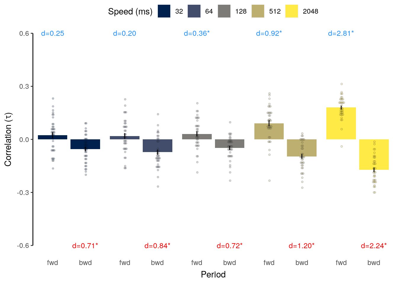
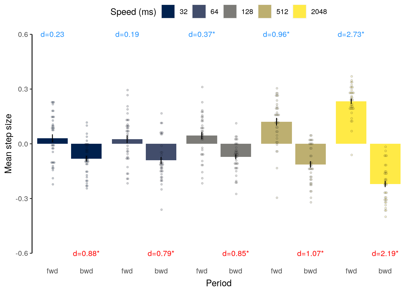
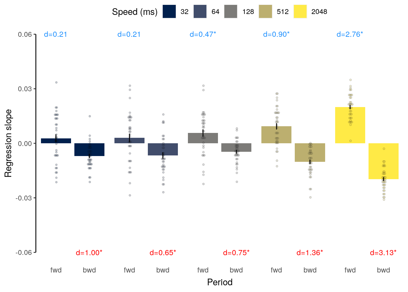
2.7.6.2 Source Data File Fig. 3e / S5b / S5d
dt_pred_seq_cor %>%
select(-classification, -num_trials, -color) %>%
write.csv(., file = file.path(path_sourcedata, "source_data_figure_3c.csv"),
row.names = FALSE)
dt_pred_seq_cor %>%
select(-classification, -num_trials, -color) %>%
write.csv(., file = file.path(path_sourcedata, "source_data_figure_s5b.csv"),
row.names = FALSE)
dt_pred_seq_cor %>%
select(-classification, -num_trials, -color) %>%
write.csv(., file = file.path(path_sourcedata, "source_data_figure_s5d.csv"),
row.names = FALSE)2.7.6.3 Source Data File Fig. S5b
dt_pred_seq_cor %>%
select(-classification, -num_trials) %>%
write.csv(., file = file.path(path_sourcedata, "source_data_figure_3c.csv"),
row.names = FALSE)2.7.6.4 Source Data File Fig. S5c
dt_pred_seq_cor %>%
select(-classification, -num_trials) %>%
write.csv(., file = file.path(path_sourcedata, "source_data_figure_3c.csv"),
row.names = FALSE)We repeat the same calculations, just splitting up the data by the serial position of the cued image:
seq_test_period_cue <- function(data, variable){
data_out = data %>%
# filter out the excluded time period (select only forward and backward period):
filter(period != "excluded") %>% setDT(.) %>%
# average for each time period and speed condition for every participant:
.[, by = .(classification, id, tITI, period, cue_pos_label), .(
mean_variable = mean(get(variable)))] %>%
# average across participants for every speed at every TR:
# check if the number of participants matches:
.[, by = .(classification, tITI, period, cue_pos_label), {
# perform a two-sided one-sample t-test against zero (baseline):
ttest_results = t.test(mean_variable, alternative = "two.sided", mu = 0);
list(
num_subs = .N,
mean_variable = mean(mean_variable),
pvalue = ttest_results$p.value,
tvalue = round(abs(ttest_results$statistic), 2),
df = ttest_results$parameter,
cohens_d = abs(round((mean(mean_variable) - 0) / sd(mean_variable), 2)),
sem_upper = mean(mean_variable) + (sd(mean_variable)/sqrt(.N)),
sem_lower = mean(mean_variable) - (sd(mean_variable)/sqrt(.N))
)
}] %>% verify(all(num_subs == 36)) %>% verify(all((num_subs - df) == 1)) %>%
# adjust p-values for multiple comparisons:
# check if the number of comparisons matches expectations:
.[period %in% c("forward", "backward"), by = .(classification), ":=" (
num_comp = .N,
pvalue_adjust = p.adjust(pvalue, method = "fdr", n = .N)
)] %>% #verify(num_comp == 10) %>%
# add variable that indicates significance with stupid significance stars:
mutate(significance = ifelse(pvalue < 0.05, "*", "")) %>%
# round the original p-values according to APA manual:
mutate(pvalue_round = round_pvalues(pvalue)) %>%
# round the adjusted p-value:
mutate(pvalue_adjust_round = round_pvalues(pvalue_adjust)) %>%
# sort data table:
setorder(classification, period, tITI) %>%
# shorten the period name:
mutate(period_short = ifelse(period == "forward", "fwd", period)) %>%
transform(period_short = ifelse(period == "backward", "bwd", period_short)) %>%
mutate(color = ifelse(period_short == "fwd", "dodgerblue", "red")) %>% setDT(.)
return(data_out)
}rmarkdown::paged_table(
seq_test_period_cue(data = dt_pred_seq_cor_cue, variable = "mean_cor") %>%
filter(pvalue_adjust < 0.05, classification == "ovr"))rmarkdown::paged_table(
seq_test_period_cue(data = dt_pred_seq_cor_cue, variable = "mean_step") %>%
filter(pvalue_adjust < 0.05, classification == "ovr"))rmarkdown::paged_table(
seq_test_period_cue(data = dt_pred_seq_cor_cue, variable = "mean_slope") %>%
filter(pvalue_adjust < 0.05, classification == "ovr"))We plot the same data, just splitting up the data by the serial position of the cued image:
plot_seq_cor_period_cue = function(data, variable){
# select the variable of interest, determine y-axis label and adjust axis:
if (variable == "mean_slope") {
ylabel = "Regression slope"
adjust_axis = 0.1
} else if (variable == "mean_cor") {
ylabel = expression("Correlation ("*tau*")")
adjust_axis = 1
} else if (variable == "mean_step") {
ylabel = "Mean step size"
adjust_axis = 1
}
dt_forward = data.table(xmin = 0, xmax = 5.5, ymin = 0, ymax = 0.4 * adjust_axis)
dt_backward = data.table(xmin = 0, xmax = 5.5, ymin = 0, ymax = -0.4 * adjust_axis)
# average across participants for every speed at every TR:
plot_data = data %>% setDT(.) %>%
.[, by = .(classification, id, tITI, period_short, cue_pos_label), .(
mean_variable = mean(get(variable))
)] %>% filter(classification == "ovr" & period_short != "excluded")
plot_stat = seq_test_period_cue(data = data, variable = variable)
# plot average correlation or betas for each speed condition and time period:
plot = ggplot(data = plot_data, aes(
x = fct_rev(as.factor(period_short)), y = as.numeric(mean_variable),
fill = as.factor(as.numeric(tITI) * 1000))) +
geom_bar(stat = "summary", fun = "mean", width = 0.9, show.legend = TRUE) +
geom_dotplot(binaxis = "y", stackdir = "center", stackratio = 0.5, alpha = 0.2,
binwidth = 0.01 * adjust_axis, show.legend = FALSE) +
geom_errorbar(stat = "summary", fun.data = "mean_se", width = 0.0, color = "black") +
geom_text(data = subset(plot_stat, classification == "ovr"), aes(
x = fct_rev(as.factor(period_short)), y = round_updown(as.numeric(mean_variable), 0.5 * adjust_axis),
label = paste0("d=", cohens_d, significance)), size = 3.0, show.legend = FALSE,
color = subset(plot_stat, classification == "ovr")$color) +
facet_grid(rows = vars(cue_pos_label),
cols = vars(as.factor(as.numeric(tITI) * 1000))) +
xlab("Period") + ylab(ylabel) +
scale_fill_viridis(name = "Speed (ms)", discrete = TRUE, option = "cividis") +
coord_capped_cart(left = "both", bottom = "both", expand = TRUE, ylim = c(-0.6, 0.6) * adjust_axis) +
theme(panel.border = element_blank(), axis.line = element_line()) +
theme(axis.line = element_line(colour = "black"),
panel.grid.major = element_blank(),
panel.grid.minor = element_blank(),
panel.border = element_blank(),
panel.background = element_blank()) +
#theme(axis.ticks.x = element_blank(), axis.line.x = element_blank()) +
theme(legend.position = "top", legend.direction = "horizontal", legend.box = "vertical",
legend.justification = "center", legend.margin = margin(t = 0, r = 0, b = 0, l = 0),
legend.box.margin = margin(t = 0, r = 0, b = -5, l = 0))
#theme(panel.spacing = unit(0, "lines"), strip.background = element_blank(),
# strip.placement = "outside", strip.text = element_blank())
return(plot)
}
fig_seq_cor_period_cue = plot_seq_cor_period_cue(data = dt_pred_seq_cor_cue, variable = "mean_cor")
fig_seq_slope_period_cue = plot_seq_cor_period_cue(data = dt_pred_seq_cor_cue, variable = "mean_slope")
fig_seq_step_period_cue = plot_seq_cor_period_cue(data = dt_pred_seq_cor_cue, variable = "mean_step")
fig_seq_cor_period_cue; fig_seq_step_period_cue; fig_seq_slope_period_cue;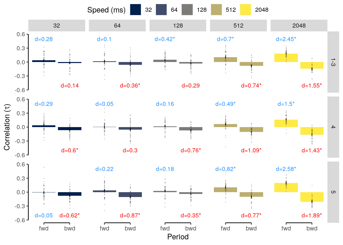
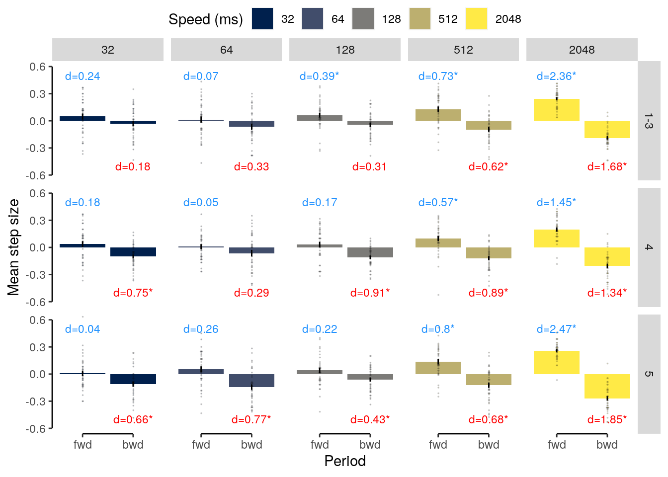
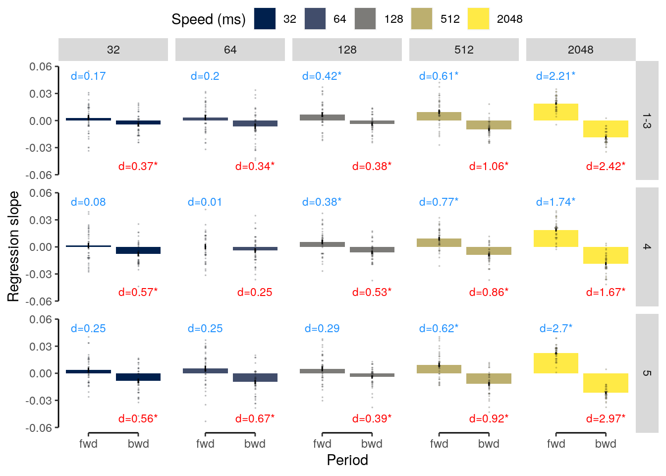
Combine plots for cue period:
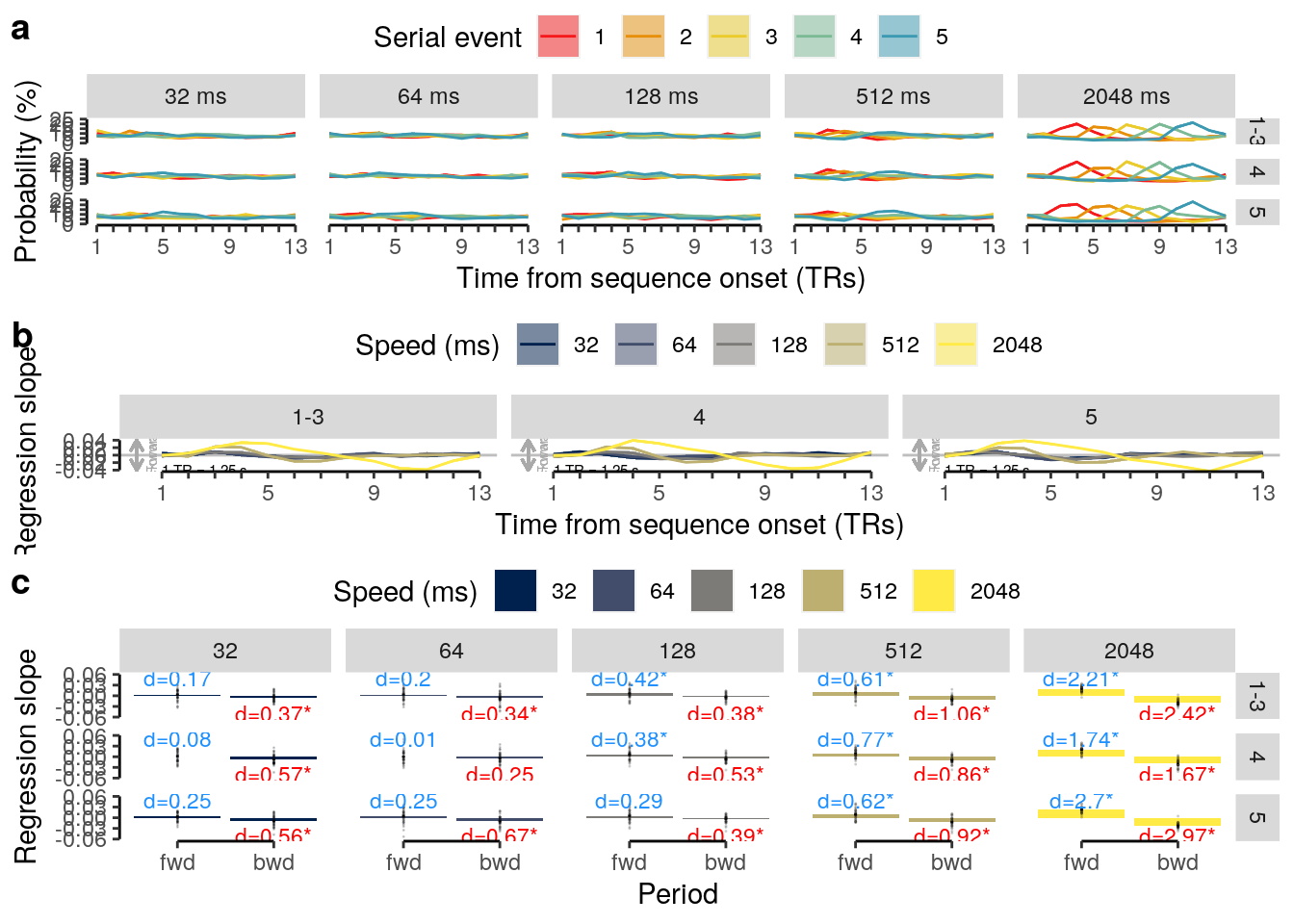
# create a data frame with the relevant data to run the LME:
lme_seq_cor_data = dt_pred_seq_cor %>%
filter(classification == "ovr" & period != "excluded") %>%
transform(tITI = as.factor(tITI))
# define linear mixed effects model with by-participant random intercepts:
lme_seq_cor = lmer(mean_slope ~ tITI * period + (1|id),
data = lme_seq_cor_data, na.action = na.omit, control = lcctrl)
summary(lme_seq_cor)## Linear mixed model fit by REML. t-tests use Satterthwaite's method [
## lmerModLmerTest]
## Formula: mean_slope ~ tITI * period + (1 | id)
## Data: lme_seq_cor_data
## Control: lcctrl
##
## REML criterion at convergence: -7231.9
##
## Scaled residuals:
## Min 1Q Median 3Q Max
## -3.8317 -0.6639 -0.0140 0.6540 3.3043
##
## Random effects:
## Groups Name Variance Std.Dev.
## id (Intercept) 7.510e-06 0.00274
## Residual 3.104e-04 0.01762
## Number of obs: 1404, groups: id, 36
##
## Fixed effects:
## Estimate Std. Error df t value Pr(>|t|)
## (Intercept) -7.007e-03 1.756e-03 9.090e+02 -3.991 7.11e-05 ***
## tITI0.064 3.263e-04 2.398e-03 1.359e+03 0.136 0.89177
## tITI0.128 2.314e-03 2.243e-03 1.359e+03 1.032 0.30234
## tITI0.512 -3.238e-03 2.243e-03 1.359e+03 -1.444 0.14898
## tITI2.048 -1.266e-02 2.076e-03 1.359e+03 -6.098 1.40e-09 ***
## periodforward 9.762e-03 2.398e-03 1.359e+03 4.072 4.94e-05 ***
## tITI0.064:periodforward -1.205e-04 3.391e-03 1.359e+03 -0.036 0.97166
## tITI0.128:periodforward 6.389e-04 3.283e-03 1.359e+03 0.195 0.84573
## tITI0.512:periodforward 9.803e-03 3.172e-03 1.359e+03 3.091 0.00204 **
## tITI2.048:periodforward 2.986e-02 2.936e-03 1.359e+03 10.170 < 2e-16 ***
## ---
## Signif. codes: 0 '***' 0.001 '**' 0.01 '*' 0.05 '.' 0.1 ' ' 1
##
## Correlation of Fixed Effects:
## (Intr) tITI0.064 tITI0.128 tITI0.512 tITI2.048 prdfrw tITI0.064:
## tITI0.064 -0.683
## tITI0.128 -0.730 0.535
## tITI0.512 -0.730 0.535 0.571
## tITI2.048 -0.788 0.577 0.617 0.617
## periodfrwrd -0.683 0.500 0.535 0.535 0.577
## tITI0.064:p 0.483 -0.707 -0.378 -0.378 -0.408 -0.707
## tITI0.128:p 0.499 -0.365 -0.683 -0.390 -0.422 -0.730 0.516
## tITI0.512:p 0.516 -0.378 -0.404 -0.707 -0.436 -0.756 0.535
## tITI2.048:p 0.557 -0.408 -0.436 -0.436 -0.707 -0.816 0.577
## tITI0.128: tITI0.512:
## tITI0.064
## tITI0.128
## tITI0.512
## tITI2.048
## periodfrwrd
## tITI0.064:p
## tITI0.128:p
## tITI0.512:p 0.552
## tITI2.048:p 0.596 0.617anova(lme_seq_cor)## Type III Analysis of Variance Table with Satterthwaite's method
## Sum Sq Mean Sq NumDF DenDF F value Pr(>F)
## tITI 0.001393 0.000348 4 1359 1.1219 0.3445
## period 0.103680 0.103680 1 1359 334.0077 <2e-16 ***
## tITI:period 0.058332 0.014583 4 1359 46.9793 <2e-16 ***
## ---
## Signif. codes: 0 '***' 0.001 '**' 0.01 '*' 0.05 '.' 0.1 ' ' 1emmeans_results = emmeans(lme_seq_cor, list(pairwise ~ period | tITI))
emmeans_pvalues = round_pvalues(summary(emmeans_results[[2]])$p.value)2.7.7 Serial target position
We calculate the average serial position at each TR:
dt_pred_seq_pos = dt_pred_seq %>%
# get the position with the highest probability at every TR:
.[, by = .(classification, id, period, tITI, trial_tITI, seq_tr), .(
num_positions = .N,
max_position = position[which.max(probability_norm)]
)] %>%
# verify that the number of position per TR matches:
verify(all(num_positions == 5)) %>%
# average the maximum position across trials for each speed condition:
.[, by = .(classification, id, period, tITI, seq_tr), .(
num_trials = .N,
mean_position = mean(max_position)
)] %>%
# verify that the number of trials per participant is correct:
verify(all(num_trials == 15)) %>%
# calculate the difference of the mean position from baseline (which is 3)
mutate(position_diff = mean_position - 3) %>%
setDT(.) %>%
# set the speed condition and period variable to a factorial variable:
transform(tTII = as.factor(tITI)) %>%
transform(period = as.factor(period))We calculate whether the average serial position is significantly different from baseline separately for every speed and period (forward vs. backward):
dt_pred_seq_pos_period = dt_pred_seq_pos %>%
# focus on the forward and backward period only:
filter(period != "excluded") %>% setDT(.) %>%
# average the mean position across trs for each period and speed condition:
.[, by = .(classification, id, period, tITI), .(
position_diff = mean(position_diff)
)] %>%
# average across participants for each speed condition and volume:
.[, by = .(classification, period, tITI), {
ttest_results = t.test(position_diff, alternative = "two.sided", mu = 0)
list(
num_subs = .N,
tvalue = round(ttest_results$statistic, 2),
pvalue = ttest_results$p.value,
df = ttest_results$parameter,
cohens_d = abs(round((mean(position_diff) - 0) / sd(position_diff), 2)),
position_diff = mean(position_diff),
conf_lb = round(ttest_results$conf.int[1], 2),
conf_ub = round(ttest_results$conf.int[2], 2),
sd_position = sd(position_diff),
sem_upper = mean(position_diff) + (sd(position_diff)/sqrt(.N)),
sem_lower = mean(position_diff) - (sd(position_diff)/sqrt(.N))
)
}] %>% verify(all(num_subs == 36)) %>%
# adjust p-values for multiple comparisons:
.[, by = .(classification), ":=" (
num_comp = .N,
pvalue_adjust = p.adjust(pvalue, method = "fdr", n = .N)
)] %>%
verify(all(num_comp == 10)) %>%
# add variable that indicates significance with stupid significance stars:
mutate(significance = ifelse(pvalue_adjust < 0.05, "*", "")) %>%
# round the original p-values:
mutate(pvalue_round = round_pvalues(pvalue)) %>%
# round the p-values adjusted for multiple comparisons:
mutate(pvalue_adjust_round = round_pvalues(pvalue_adjust)) %>%
# sort the datatable for each speed and TR:
setorder(., classification, period, tITI) %>%
# shorten the period name:
mutate(period_short = ifelse(period == "forward", "fwd", period)) %>%
transform(period_short = ifelse(period == "backward", "bwd", period_short)) %>%
mutate(color = ifelse(period_short == "fwd", "dodgerblue", "red")) %>% setDT(.)
dt_pred_seq_pos_period %>%
filter(classification == "ovr", pvalue_adjust < 0.05) %>%
rmarkdown::paged_table(.)We calculate the mean serial position at every TR and compare it against baseline:
dt_pred_seq_pos_tr = dt_pred_seq_pos %>%
# average across participants for each speed condition and volume:
.[, by = .(classification, period, tITI, seq_tr), {
ttest_results = t.test(mean_position, alternative = "two.sided", mu = 3)
list(
num_subs = .N,
tvalue = ttest_results$statistic,
pvalue = ttest_results$p.value,
df = ttest_results$parameter,
mean_position = mean(mean_position),
sd_position = sd(mean_position),
sem_upper = mean(mean_position) + (sd(mean_position)/sqrt(.N)),
sem_lower = mean(mean_position) - (sd(mean_position)/sqrt(.N))
)
}] %>% verify(all(num_subs == 36)) %>%
# adjust p-values for multiple comparisons:
.[period %in% c("forward", "backward"), by = .(classification), ":=" (
num_comp = .N,
pvalue_adjust = p.adjust(pvalue, method = "fdr", n = .N)
)] %>% verify(all(num_comp == 39, na.rm = TRUE)) %>%
# round the original p-values:
mutate(pvalue_rounded = round_pvalues(pvalue)) %>%
# round the p-values adjusted for multiple comparisons:
mutate(pvalue_adjust_rounded = round_pvalues(pvalue_adjust)) %>%
#
mutate(significance = ifelse(pvalue_adjust < 0.05, "***", "")) %>%
# sort the datatable for each speed and TR:
setorder(., classification, period, tITI, seq_tr)
dt_pred_seq_pos_tr %>%
filter(classification == "ovr", pvalue_adjust < 0.05) %>%
rmarkdown::paged_table(.)cfg = list(variable = "mean_position", threshold = 2.021, baseline = 3,
grouping = c("classification", "tITI"), n_perms = 10000, n_trs = 13)
dt_pred_seq_pos_cluster = cluster_permutation(dt_pred_seq_pos_sub, cfg)# define linear mixed effects model with by-participant random intercepts:
lme_seq_pos = lmer(position_diff ~ tITI * period + (1 + tITI + period |id),
data = subset(dt_pred_seq_pos, classification == "ovr" & period != "excluded"),
na.action = na.omit, control = lcctrl)## Warning: Model failed to converge with 2 negative eigenvalues: -1.2e-01 -4.0e+01summary(lme_seq_pos)## Linear mixed model fit by REML. t-tests use Satterthwaite's method [
## lmerModLmerTest]
## Formula: position_diff ~ tITI * period + (1 + tITI + period | id)
## Data:
## subset(dt_pred_seq_pos, classification == "ovr" & period != "excluded")
## Control: lcctrl
##
## REML criterion at convergence: 1843
##
## Scaled residuals:
## Min 1Q Median 3Q Max
## -3.1107 -0.7007 0.0074 0.6663 3.2056
##
## Random effects:
## Groups Name Variance Std.Dev. Corr
## id (Intercept) 0.000000 0.00000
## tITI0.064 0.001009 0.03177 NaN
## tITI0.128 0.000316 0.01778 NaN 1.00
## tITI0.512 0.008749 0.09354 NaN 1.00 1.00
## tITI2.048 0.013608 0.11665 NaN 1.00 1.00 1.00
## periodforward 0.066908 0.25867 NaN -1.00 -1.00 -1.00 -1.00
## Residual 0.203320 0.45091
## Number of obs: 1404, groups: id, 36
##
## Fixed effects:
## Estimate Std. Error df t value Pr(>|t|)
## (Intercept) 2.130e-01 4.339e-02 1.359e+03 4.908 1.03e-06 ***
## tITI0.064 -1.790e-02 6.159e-02 1.025e+03 -0.291 0.771373
## tITI0.128 -7.824e-02 5.747e-02 1.199e+03 -1.361 0.173671
## tITI0.512 5.000e-02 5.948e-02 3.345e+02 0.841 0.401142
## tITI2.048 2.917e-01 5.659e-02 2.100e+02 5.154 5.86e-07 ***
## periodforward -2.346e-01 7.499e-02 1.810e+02 -3.128 0.002052 **
## tITI0.064:periodforward -7.407e-03 8.678e-02 1.359e+03 -0.085 0.931987
## tITI0.128:periodforward -1.543e-04 8.402e-02 1.359e+03 -0.002 0.998535
## tITI0.512:periodforward -2.710e-01 8.117e-02 1.359e+03 -3.338 0.000865 ***
## tITI2.048:periodforward -8.142e-01 7.515e-02 1.359e+03 -10.834 < 2e-16 ***
## ---
## Signif. codes: 0 '***' 0.001 '**' 0.01 '*' 0.05 '.' 0.1 ' ' 1
##
## Correlation of Fixed Effects:
## (Intr) tITI0.064 tITI0.128 tITI0.512 tITI2.048 prdfrw tITI0.064:
## tITI0.064 -0.704
## tITI0.128 -0.755 0.536
## tITI0.512 -0.730 0.536 0.564
## tITI2.048 -0.767 0.570 0.597 0.649
## periodfrwrd -0.579 0.358 0.407 0.271 0.246
## tITI0.064:p 0.500 -0.704 -0.377 -0.365 -0.383 -0.579
## tITI0.128:p 0.516 -0.364 -0.682 -0.377 -0.396 -0.598 0.516
## tITI0.512:p 0.535 -0.377 -0.404 -0.682 -0.410 -0.619 0.535
## tITI2.048:p 0.577 -0.407 -0.436 -0.421 -0.664 -0.668 0.577
## tITI0.128: tITI0.512:
## tITI0.064
## tITI0.128
## tITI0.512
## tITI2.048
## periodfrwrd
## tITI0.064:p
## tITI0.128:p
## tITI0.512:p 0.552
## tITI2.048:p 0.596 0.617anova(lme_seq_pos)## Type III Analysis of Variance Table with Satterthwaite's method
## Sum Sq Mean Sq NumDF DenDF F value Pr(>F)
## tITI 2.000 0.4999 4 191.31 2.4588 0.04694 *
## period 16.834 16.8338 1 36.86 82.7945 5.831e-11 ***
## tITI:period 43.623 10.9056 4 1358.61 53.6377 < 2.2e-16 ***
## ---
## Signif. codes: 0 '***' 0.001 '**' 0.01 '*' 0.05 '.' 0.1 ' ' 1emmeans_results = emmeans(lme_seq_pos, list(pairwise ~ period | tITI))
emmeans_pvalues = round_pvalues(summary(emmeans_results[[2]])$p.value)2.7.7.1 Figure 3g
variable = "position_diff"
plot_data = dt_pred_seq_pos %>%
# average across participants for every speed at every TR:
.[, by = .(classification, id, tITI, period), .(
mean_variable = mean(get(variable))
)] %>%
filter(classification == "ovr" & period != "excluded") %>%
# shorten the period name:
mutate(period_short = ifelse(period == "forward", "fwd", period)) %>%
transform(period_short = ifelse(period == "backward", "bwd", period_short)) %>%
mutate(color = ifelse(period_short == "fwd", "dodgerblue", "red")) %>%
setDT(.)
# plot average correlation or betas for each speed condition and time period:
fig_seq_pos_period = ggplot(data = plot_data, aes(
x = fct_rev(as.factor(period_short)), y = as.numeric(mean_variable),
fill = as.factor(as.numeric(tITI) * 1000))) +
geom_bar(stat = "summary", fun = "mean", width = 0.9, show.legend = TRUE) +
geom_dotplot(binaxis = "y", stackdir = "center", stackratio = 0.5, alpha = 0.2,
binwidth = 0.05, show.legend = FALSE) +
geom_errorbar(stat = "summary", fun.data = "mean_se", width = 0.0, color = "black") +
geom_text(data = subset(dt_pred_seq_pos_period, classification == "ovr"), aes(
x = fct_rev(as.factor(period_short)), y = round_updown(as.numeric(get(variable)), 1.2),
label = paste0("d=", sprintf("%.2f", cohens_d), significance)), show.legend = FALSE, size = 3.2,
color = subset(dt_pred_seq_pos_period, classification == "ovr")$color) +
facet_wrap(~ as.factor(as.numeric(tITI) * 1000), strip.position = "bottom", nrow = 1) +
xlab("Period") + ylab("Event position\ncompared to baseline") +
scale_colour_viridis(name = "Speed (ms)", discrete = TRUE, option = "cividis") +
scale_fill_viridis(name = "Speed (ms)", discrete = TRUE, option = "cividis") +
coord_capped_cart(left = "both", bottom = "both", expand = TRUE, ylim = c(-1.5, 1.5)) +
theme(legend.position = "top", legend.direction = "horizontal",
legend.justification = "center", legend.margin = margin(t = 0, r = 0, b = 0, l = 0),
legend.box.margin = margin(t = 0, r = 0, b = 0, l = 0)) +
theme(panel.spacing = unit(0, "lines"), strip.background = element_blank(),
strip.placement = "outside", strip.text = element_blank()) +
theme(axis.ticks.x = element_line(colour = "white"),
axis.line.x = element_line(colour = "white")) +
theme(axis.line.y = element_line(colour = "black"),
panel.grid.major = element_blank(),
panel.grid.minor = element_blank(),
panel.border = element_blank(),
panel.background = element_blank())
fig_seq_pos_period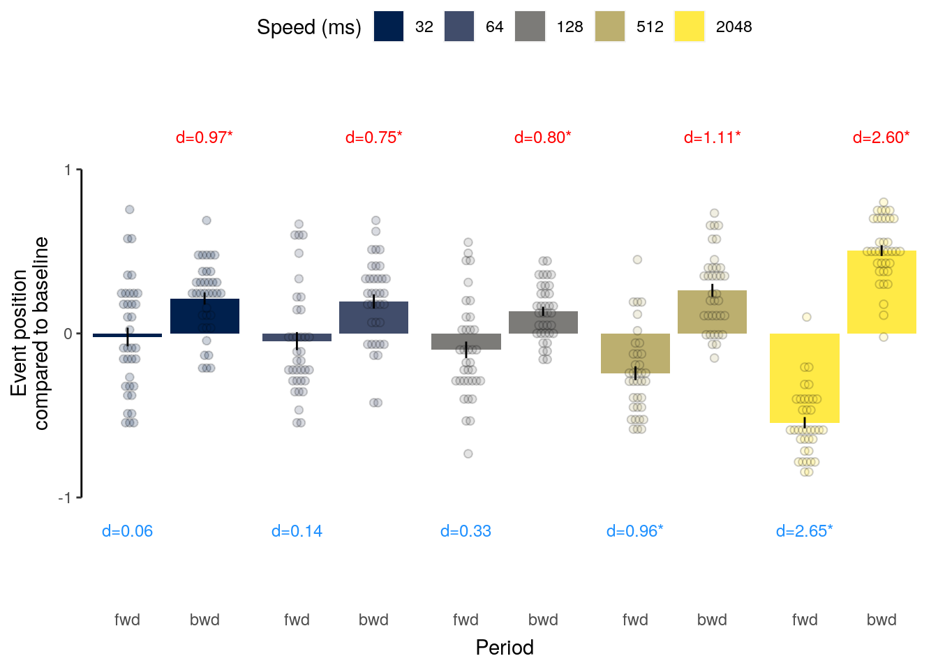
2.7.7.2 Source Data File Fig. 3g
subset(plot_data, classification == "ovr") %>%
select(-classification, -color) %>%
write.csv(., file = file.path(path_sourcedata, "source_data_figure_3g.csv"),
row.names = FALSE)2.7.7.3 Figure 3f
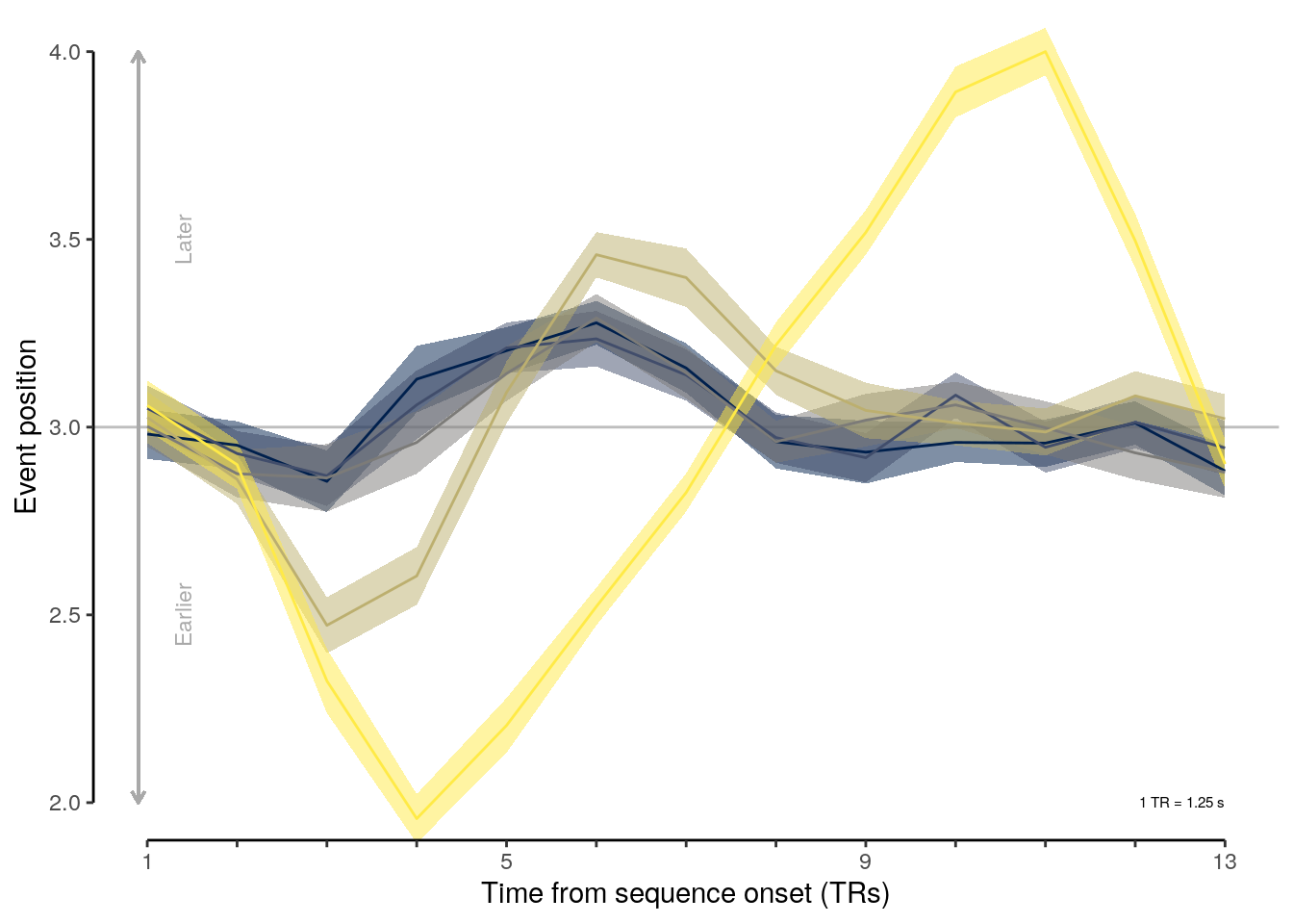
2.7.7.4 Source Data File Fig. 3f
subset(dt_pred_seq_pos_tr, classification == "ovr") %>%
select(-classification, -num_subs, -num_comp, -pvalue_adjust,
-pvalue_rounded, -pvalue_adjust_rounded, -pvalue, -df,
-tvalue, -significance, -sd_position) %>%
write.csv(., file = file.path(path_sourcedata, "source_data_figure_3f.csv"),
row.names = FALSE)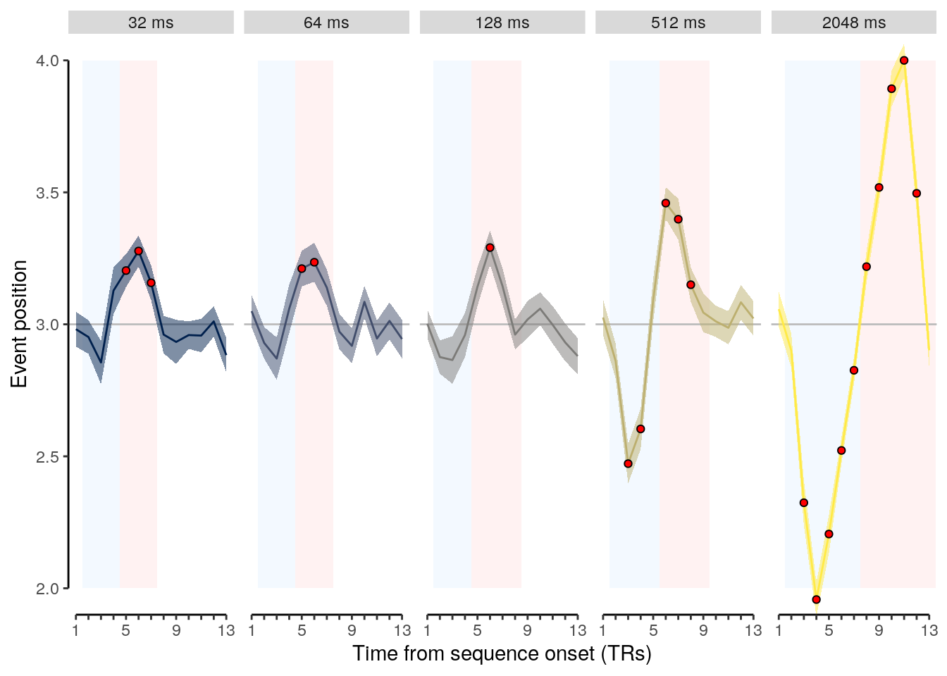
2.7.8 Transititons
We calculate the step size between consecutively decoded (highest probability) events:
dt_pred_seq_step = dt_pred_seq %>%
# get the position with the highest probability for every TR:
.[, by = .(classification, id, tITI, trial_tITI, seq_tr), ":=" (
num_classes = .N,
rank_order = rank(-probability),
max_prob = as.numeric(probability == max(probability))
)] %>%
# verify that there are five classes per TR:
verify(all(num_classes == 5)) %>%
# sort the data table:
setorder(., classification, id, tITI, trial_tITI, seq_tr) %>%
# select only classes with the highest probability for every TR:
filter(max_prob == 1) %>%
setDT(.) %>%
# check if the rank order of the event with highest probability match:
verify(all(rank_order == max_prob)) %>%
# group by classification, id, speed and trial and calculate step sizes:
.[, by = .(classification, id, tITI, trial_tITI),
step := position - shift(position)]We calculate the mean step size for early and late period in the forward and backward phase:
dt_pred_seq_step_mean = dt_pred_seq_step %>%
filter(period != "excluded") %>%
filter(!(is.na(zone))) %>% setDT(.) %>%
# shorten the period name:
mutate(period_short = ifelse(period == "forward", "fwd", period)) %>%
transform(period_short = ifelse(period == "backward", "bwd", period_short)) %>%
setDT(.) %>%
.[, by = .(classification, id, tITI, period_short, zone), .(
mean_step = mean(step, na.rm = TRUE))]We compare the forward and the backward period using t-tests:
dt_pred_seq_step_stat = dt_pred_seq_step_mean %>%
spread(key = period_short, value = mean_step, drop = TRUE) %>%
mutate(difference = fwd - bwd) %>% setDT(.) %>%
# average across participants for each speed condition and volume:
.[, by = .(classification, tITI, zone), {
ttest_results = t.test(fwd, bwd, alternative = "two.sided", paired = TRUE)
list(
num_subs = .N,
tvalue = round(ttest_results$statistic, 2),
pvalue = ttest_results$p.value,
df = ttest_results$parameter,
cohens_d = abs(round((mean(fwd) - mean(bwd)) / sd(fwd - bwd), 2)),
mean_step = mean(difference),
sd_step = sd(difference),
sem_upper = mean(difference) + (sd(difference)/sqrt(.N)),
sem_lower = mean(difference) - (sd(difference)/sqrt(.N))
)
}] %>% verify(all(num_subs == 36)) %>%
# adjust p-values for multiple comparisons:
.[, by = .(classification), ":=" (
num_comp = .N,
pvalue_adjust = p.adjust(pvalue, method = "fdr", n = .N)
)] %>%
verify(all(num_comp == 10)) %>%
# add variable that indicates significance with stupid significance stars:
mutate(significance = ifelse(pvalue < 0.05, "*", "")) %>%
# round the original p-values:
mutate(pvalue_round = round_pvalues(pvalue)) %>%
# round the p-values adjusted for multiple comparisons:
mutate(pvalue_adjust_round = round_pvalues(pvalue_adjust)) %>%
# sort the datatable for each speed and TR:
setorder(., classification, zone, tITI)
dt_pred_seq_step_stat %>%
filter(classification == "ovr") %>%
rmarkdown::paged_table(.)We compare each period to the baseline:
dt_pred_seq_step_stat_baseline = dt_pred_seq_step_mean %>%
# average across participants for each speed condition and volume:
.[, by = .(classification, tITI, period_short, zone), {
ttest_results = t.test(mean_step, mu = 0, alternative = "two.sided")
list(
num_subs = .N,
tvalue = round(ttest_results$statistic, 2),
pvalue = ttest_results$p.value,
df = ttest_results$parameter,
cohens_d = abs(round((mean(mean_step) - 0) / sd(mean_step), 2)),
mean_step = mean(mean_step),
sd_step = sd(mean_step),
sem_upper = mean(mean_step) + (sd(mean_step)/sqrt(.N)),
sem_lower = mean(mean_step) - (sd(mean_step)/sqrt(.N))
)
}] %>% verify(all(num_subs == 36)) %>%
# adjust p-values for multiple comparisons:
.[, by = .(classification), ":=" (
num_comp = .N,
pvalue_adjust = p.adjust(pvalue, method = "fdr", n = .N)
)] %>%
# verf
verify(all(num_comp == 20)) %>%
# add variable that indicates significance with stupid significance stars:
mutate(significance = ifelse(pvalue_adjust < 0.05, "*", "")) %>%
# round the original p-values:
mutate(pvalue_round = round_pvalues(pvalue)) %>%
# round the p-values adjusted for multiple comparisons:
mutate(pvalue_adjust_round = round_pvalues(pvalue_adjust)) %>%
# sort the datatable for each speed and TR:
setorder(., classification, period_short, zone, tITI)
dt_pred_seq_step_stat_baseline %>%
filter(classification == "ovr", pvalue < 0.05) %>%
rmarkdown::paged_table(.)2.7.8.1 Figure 3h
# plot average correlation or betas for each speed condition and time period:
fig_seq_step = ggplot(data = subset(dt_pred_seq_step_mean, classification == "ovr"), aes(
x = fct_rev(as.factor(period_short)), y = as.numeric(mean_step),
fill = as.factor(as.numeric(tITI) * 1000)), color = as.factor(as.numeric(tITI) * 1000)) +
facet_grid(vars(as.factor(zone)), vars(as.factor(as.numeric(tITI) * 1000)), switch = "x") +
geom_bar(stat = "summary", fun = "mean", width = 0.9) +
geom_point(position = position_jitterdodge(jitter.height = 0, seed = 4, jitter.width = 0.2),
pch = 21, alpha = 0.05, color = "black", show.legend = FALSE) +
geom_errorbar(stat = "summary", fun.data = "mean_se", width = 0.0, color = "black") +
geom_text(data = subset(dt_pred_seq_step_stat, classification == "ovr"), aes(
y = 2, label = paste0("d=", sprintf("%.2f", cohens_d), significance), x = 1.5),
inherit.aes = FALSE, color = "black", size = 3.3) +
xlab("Period") + ylab("Step size") +
scale_colour_viridis(discrete = TRUE, option = "cividis", name = "Speed (ms)") +
scale_fill_viridis(discrete = TRUE, option = "cividis", name = "Speed (ms)") +
coord_capped_cart(left = "both", bottom = "both", expand = TRUE, ylim = c(-2, 2)) +
theme(legend.position = "top", legend.direction = "horizontal",
legend.justification = "center", legend.margin = margin(t = 0, r = 0, b = -5, l = 0),
legend.box.margin = margin(t = 0, r = 0, b = 0, l = 0)) +
theme(panel.spacing.x = unit(0, "lines"), strip.background.x = element_blank(),
strip.placement.x = "outside", strip.text.x = element_blank()) +
theme(axis.ticks.x = element_line(colour = "white"),
axis.line.x = element_line(colour = "white")) +
#theme(axis.title.x = element_blank()) +
theme(strip.text = element_text(margin = margin(b = 2, t = 2, r = 2, l = 2))) +
theme(axis.line.y = element_line(colour = "black"),
panel.grid.major = element_blank(),
panel.grid.minor = element_blank(),
panel.border = element_blank(),
panel.background = element_blank())
fig_seq_step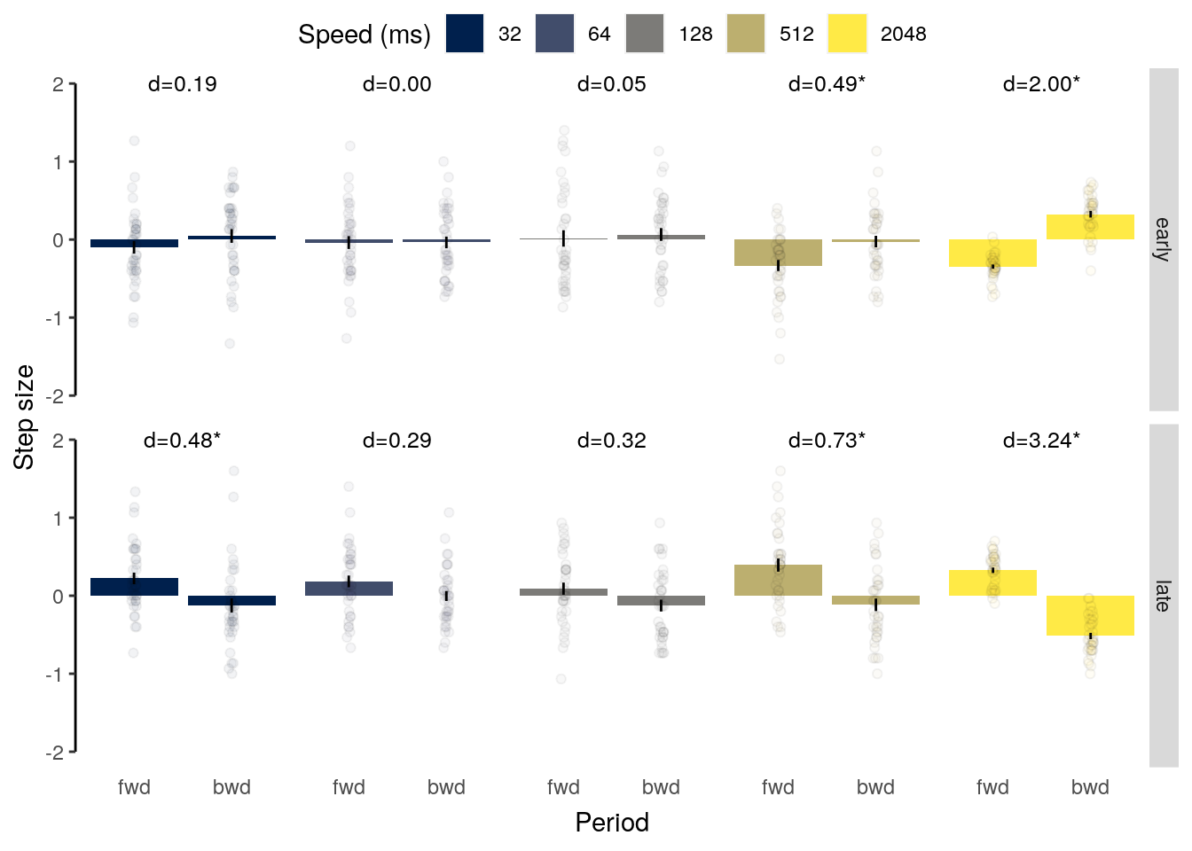
2.7.8.2 Source Data File Fig. 3h
subset(dt_pred_seq_step_mean, classification == "ovr") %>%
select(-classification) %>%
write.csv(., file = file.path(path_sourcedata, "source_data_figure_3h.csv"),
row.names = FALSE)plot_grid(fig_seq_pos_period, fig_seq_step, labels = "auto",
ncol = 2, label_fontface = "bold", rel_widths = c(5, 6))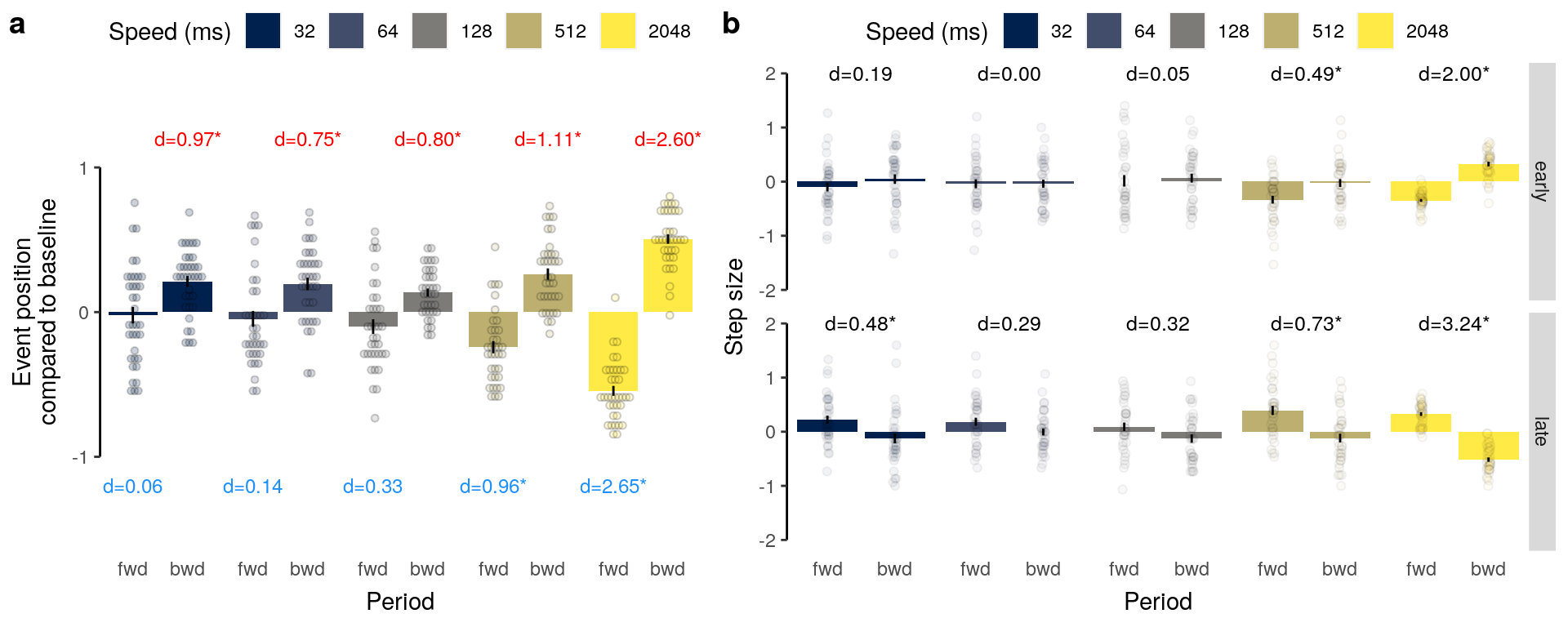
plot_grid(fig_seq_cor_time, fig_seq_cor_period, fig_seq_step_time, fig_seq_step_period,
labels = "auto", ncol = 2, nrow = 2, label_fontface = "bold")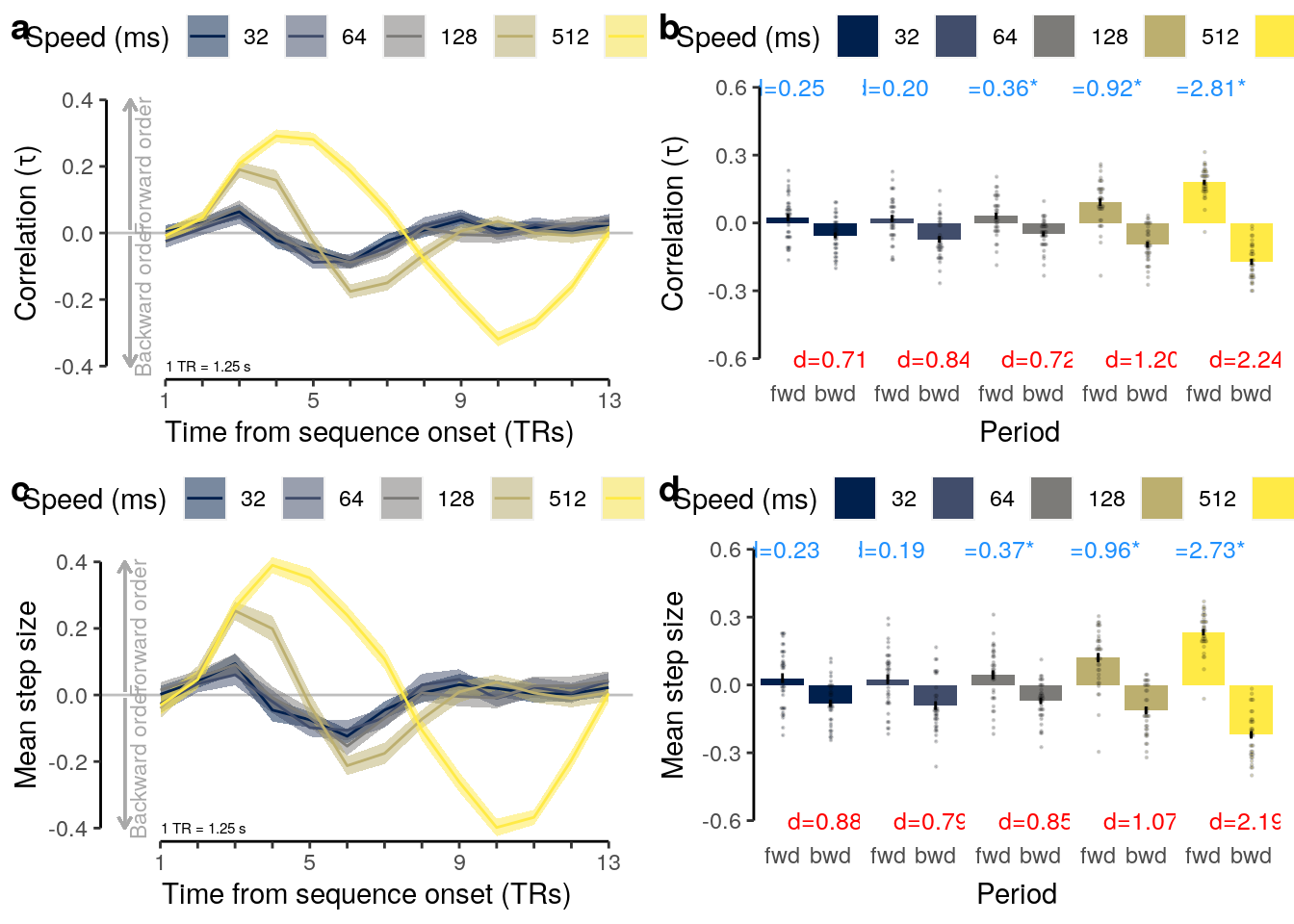
2.7.8.3 Source Data File Fig. 3f
seq_test_time(data = dt_pred_seq_cor, variable = "mean_slope") %>%
filter(pvalue_adjust < 0.05 & classification == "ovr") %>%
rmarkdown::paged_table(.)seq_test_time(data = dt_pred_seq_cor, variable = "mean_cor") %>%
filter(pvalue_adjust < 0.05 & classification == "ovr") %>%
rmarkdown::paged_table(.)seq_test_time(data = dt_pred_seq_cor, variable = "mean_step") %>%
filter(pvalue_adjust < 0.05 & classification == "ovr") %>%
rmarkdown::paged_table(.)2.7.8.4 Figure S6
fig_seq_slope_time_facet = plot_seq_cor_facet(dt = subset(
seq_test_time(data = dt_pred_seq_cor, variable = "mean_slope"),
classification == "ovr"), variable = "mean_slope")
fig_seq_cor_time_facet = plot_seq_cor_facet(dt = subset(
seq_test_time(data = dt_pred_seq_cor, variable = "mean_cor"),
classification == "ovr"), variable = "mean_cor")
fig_seq_step_time_facet = plot_seq_cor_facet(dt = subset(
seq_test_time(data = dt_pred_seq_cor, variable = "mean_step"),
classification == "ovr"), variable = "mean_step")
remove_xaxis = theme(axis.title.x = element_blank())
remove_facets = theme(strip.background = element_blank(), strip.text.x = element_blank())
plot_grid(fig_seq_slope_time_facet + remove_xaxis,
fig_seq_pos_time_facet + remove_xaxis + theme(legend.position = "none") + remove_facets,
fig_seq_cor_time_facet + remove_xaxis + theme(legend.position = "none") + remove_facets,
fig_seq_step_time_facet + theme(legend.position = "none") + remove_facets,
labels = "auto", ncol = 1, label_fontface = "bold")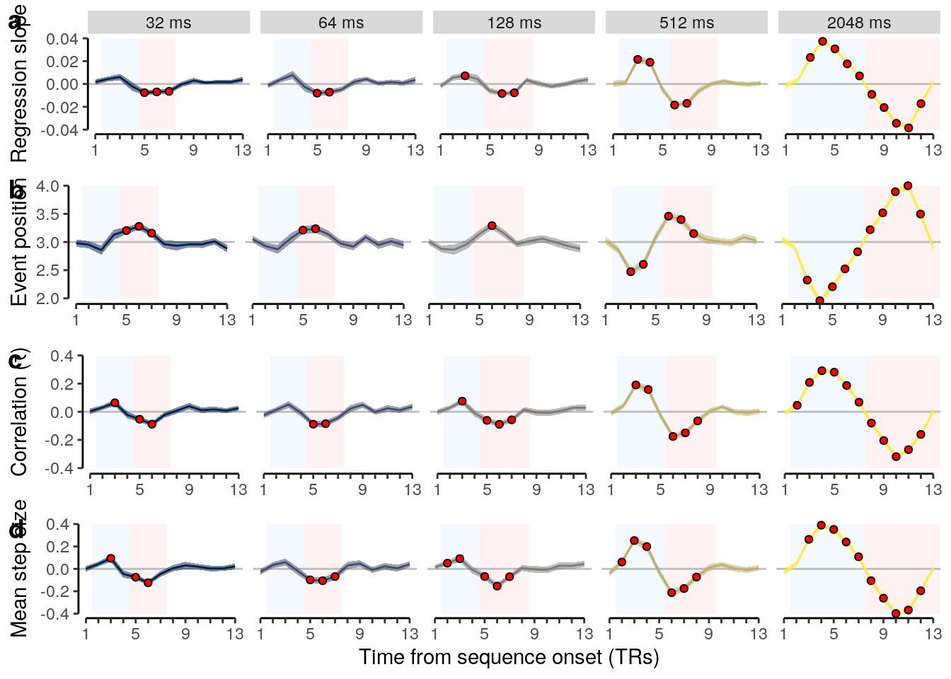
ggsave(filename = "wittkuhn_schuck_figure_s6.pdf",
plot = last_plot(), device = cairo_pdf, path = path_figures, scale = 1,
dpi = "retina", width = 7, height = 9)2.7.8.5 Source Data File Fig. S6a
subset(seq_test_time(data = dt_pred_seq_cor, variable = "mean_slope"),
classification == "ovr") %>%
select(-classification, -num_subs, -num_comp) %>%
write.csv(., file = file.path(path_sourcedata, "source_data_figure_s6a.csv"),
row.names = FALSE)2.7.8.6 Source Data File Fig. S6b
subset(dt_pred_seq_pos_tr, classification == "ovr") %>%
select(-classification, -num_subs, -num_comp) %>%
write.csv(., file = file.path(path_sourcedata, "source_data_figure_s6b.csv"),
row.names = FALSE)2.7.8.7 Source Data File Fig. S6c
subset(seq_test_time(data = dt_pred_seq_cor, variable = "mean_cor"),
classification == "ovr") %>%
select(-classification, -num_subs, -num_comp) %>%
write.csv(., file = file.path(path_sourcedata, "source_data_figure_s6c.csv"),
row.names = FALSE)2.7.8.8 Source Data File Fig. S6d
subset(seq_test_time(data = dt_pred_seq_cor, variable = "mean_step"),
classification == "ovr") %>%
select(-classification, -num_subs, -num_comp) %>%
write.csv(., file = file.path(path_sourcedata, "source_data_figure_s6d.csv"),
row.names = FALSE)2.7.9 Figure 3
Plot Figure 3 in the main text:
plot_grid(
plot_grid(fig_seq_probas, labels = c("a"), nrow = 1),
plot_grid(fig_seq_slope_time, fig_seq_slope_period, labels = c("b", "c"),
ncol = 2, nrow = 1, label_fontface = "bold", rel_widths = c(4.9, 5)),
plot_grid(fig_seq_cor_between, fig_seq_cor_within, fig_seq_pos_time,
labels = c("d", "e", "f"), ncol = 3, rel_widths = c(0.325, 0.325, 0.35)),
plot_grid(fig_seq_pos_period, fig_seq_step, labels = c("g", "h"),
ncol = 2, label_fontface = "bold", nrow = 1),
nrow = 4, label_fontface = "bold", rel_heights = c(2, 3)
)## `geom_smooth()` using formula 'y ~ x'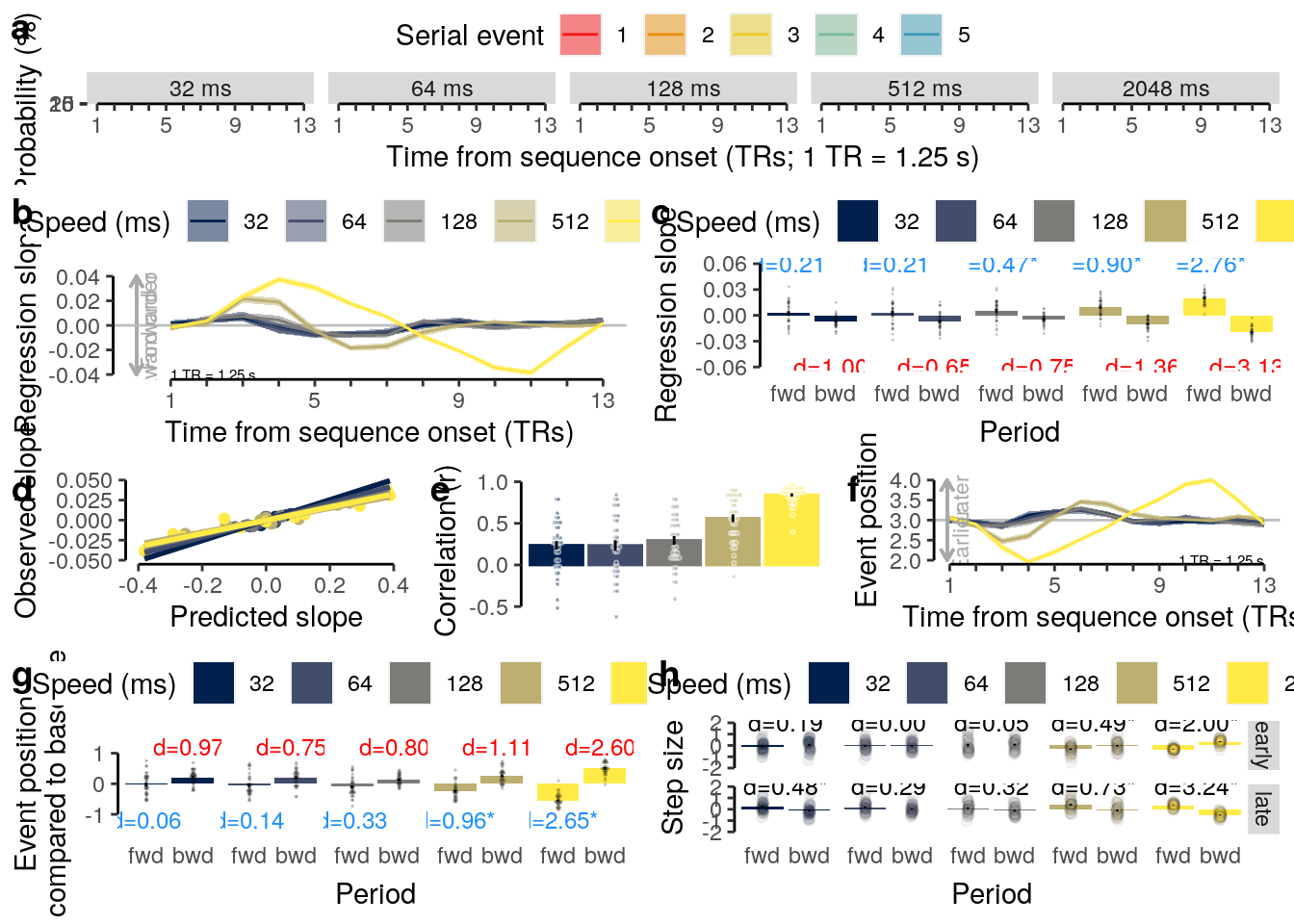
ggsave(filename = "wittkuhn_schuck_figure_3.pdf",
plot = last_plot(), device = cairo_pdf, path = path_figures, scale = 1,
dpi = "retina", width = 10, height = 12)2.7.9.1 Figure S7
2.8 Decoding: Repetition trials
2.8.1 Preparation
2.8.1.1 Initialization
We load the data and relevant functions:
# find the path to the root of this project:
if (!requireNamespace("here")) install.packages("here")
if ( basename(here::here()) == "highspeed" ) {
path_root = here::here("highspeed-analysis")
} else {
path_root = here::here()
}
# create a list of participants to exclude based on behavioral performance:
sub_exclude <- c("sub-24", "sub-31", "sub-37", "sub-40")The next step is only evaluated during manual execution:
# source all relevant functions from the setup R script:
source(file.path(path_root, "code", "highspeed-analysis-setup.R"))2.8.1.2 Prepare events and decoding data
We prepare the behavioral events data and the decoding data of repetition trials:
# create a subset of the events data table only including repetition task events:
dt_events_rep = dt_events %>%
filter(condition == "repetition" & trial_type == "stimulus") %>%
setDT(.)
# create a data table containing all classifier predictions on repetition trials:
dt_pred_rep = dt_pred %>%
# create a subset of the decoding data only including the repetition task data:
filter(condition == "repetition" & class != "other" & mask == "cv" & stim != "cue") %>%
setDT(.) %>%
# filter excluded participants:
filter(!(id %in% sub_exclude)) %>%
setDT(.) %>%
# add the serial position, change trial and target cue to the repetition data table:
.[, c("position", "change", "trial_cue") := get_pos(.SD, dt_events_rep),
by = .(id, trial, class), .SDcols = c("id", "trial", "class")] %>%
# add a counter for the number of change trials in the repetition data:
.[, by = .(id, classifier, class, change), ":=" (
trial_change = rep(1:length(unique(trial)), each = max(seq_tr))
)] %>%
# add random position indices for out-of-class stimuli:
.[is.na(position), by = .(id, classification, trial), ":=" (
position = rep(permute(3:5), each = max(seq_tr))
)] %>%
# check if there are any NA values:
verify(!is.na(position)) %>%
# create a new variable containing the position label by copying the position:
mutate(position_label = position) %>%
# re-label all positions > 2 to "other":
transform(position_label = ifelse(position_label > 2, "none", position_label)) %>%
setDT(.) %>%
# create a new variable counting the occurrence of each event position:
.[position != 2, ":=" (occurence = change - 1)] %>%
.[position == 2 & change <= 9, ":=" (occurence = max(change) + 1 - change)] %>%
.[position == 2 & change == 16, ":=" (occurence = max(change) + 1 - change)]2.8.2 Probability time-courses
First, we average across trials for each factor grouping and calculate the mean classification probability for each serial event. Note, that this approach averages across the specific stimuli used in any given trial as the specific stimulus identities are not considered important here. We verify if the correct number of trials was used for the calculations. Next, we average across participants. We calculate the average probability of each serial event and also calculate the standard error of them mean.
dt_pred_rep_timecourses = dt_pred_rep %>%
# calculate the mean probability for every repetition condition and TR
.[, by = .(classification, id, seq_tr, change, position), .(
num_events = .N,
mean_probability = mean(probability * 100)
)] %>% verify(num_events == 5) %>%
# average mean probability across participants:
.[, by = .(classification, seq_tr, change, position), .(
num_sub = .N,
mean_probability = mean(mean_probability),
sem_upper = mean(mean_probability) + (sd(mean_probability)/sqrt(.N)),
sem_lower = mean(mean_probability) - (sd(mean_probability)/sqrt(.N))
)] %>%
verify(all(num_sub == 36))We define the colors used for plotting as well as the facet labels:
# define colors for plotting:
colors_inseq = colorRampPalette(c("dodgerblue", "red"), space = "Lab")(2)
colors_outseq = colorRampPalette(c("gray70", "gray90"), alpha = TRUE)(3)
colors = c(colors_inseq, colors_outseq)
# change the facet labels such that it shows the time-point of the change from
# the first to the second unique stimulus:
facet_labels_new = c(sort(unique(paste0(dt_pred_rep_timecourses$change[
dt_pred_rep_timecourses$change != 16]-1, "/", 10-dt_pred_rep_timecourses$change[
dt_pred_rep_timecourses$change != 16]))), unique(paste0(dt_pred_rep_timecourses$change[
dt_pred_rep_timecourses$change == 16]-1, "/1")))
facet_labels_new[1] = paste("short", sprintf('\u2192'), "long")
facet_labels_new[1] = "Forward interference"
facet_labels_new[length(facet_labels_new)-1] = "Backward interference"
facet_labels_old = as.character(sort(unique(dt_pred_rep_timecourses$change)))
names(facet_labels_new) = facet_labels_old2.8.2.1 Figure 4a
We plot the probability time courses:
trs = c(2, 7)
plot_rep_probas <- function(data, xmin = 1, xmax = 13) {
# reduced the data frame to plot rectangles (see below):
data_factor_reduced = subset(data, position == 1 & seq_tr == 1)
ggplot(data, aes(x = as.numeric(seq_tr), y = as.numeric(mean_probability),
color = as.factor(position), fill = as.factor(position))) +
facet_wrap(~ as.factor(change), ncol = 3, labeller = as_labeller(facet_labels_new)) +
geom_rect(data = data_factor_reduced, fill = "gray", alpha = 0.15, color = NA,
aes(xmin = xmin, xmax = xmax, ymin = 0, ymax = 60)) +
geom_ribbon(aes(ymin = sem_lower, ymax = sem_upper), alpha = 0.5, color = NA) +
geom_line() +
xlab("Time from sequence onset (TRs)") + ylab("Probability (%)") +
annotate("text", x = 13, y = 0, label = "1 TR = 1.25 s",
hjust = 1, size = rel(2)) +
scale_colour_manual(name = "Serial event", values = colors) +
scale_fill_manual(name = "Serial event", values = colors) +
scale_x_continuous(labels = label_fill(seq(1,13,1), mod = 4), breaks = seq(1,13,1)) +
coord_capped_cart(left = "both", bottom = "both", ylim = c(0,60)) +
theme(strip.text.x = element_text(margin = margin(b = 3, t = 2))) +
guides(color = guide_legend(nrow = 1)) +
theme(legend.position = "bottom", legend.direction = "horizontal",
legend.justification = "center", legend.margin = margin(0,0,0,0),
legend.box.margin = margin(t = -5, r = 0, b = 10, l = 0)) +
theme(panel.background = element_blank()) +
theme(axis.line = element_line(colour = "black"),
panel.grid.major = element_blank(),
panel.grid.minor = element_blank(),
panel.border = element_blank(),
panel.background = element_blank())
}
plot_data = dt_pred_rep_timecourses %>% filter(classification == "ovr" & change %in% c(2,9))
fig_a = plot_rep_probas(data = plot_data, xmin = trs[1] - 0.5, xmax = trs[2] + 0.5)
fig_s1_a = plot_rep_probas(data = subset(dt_pred_rep_timecourses, classification == "ovr"),
xmin = trs[1] - 0.5, xmax = trs[2] + 0.5)
fig_a; fig_s1_a; 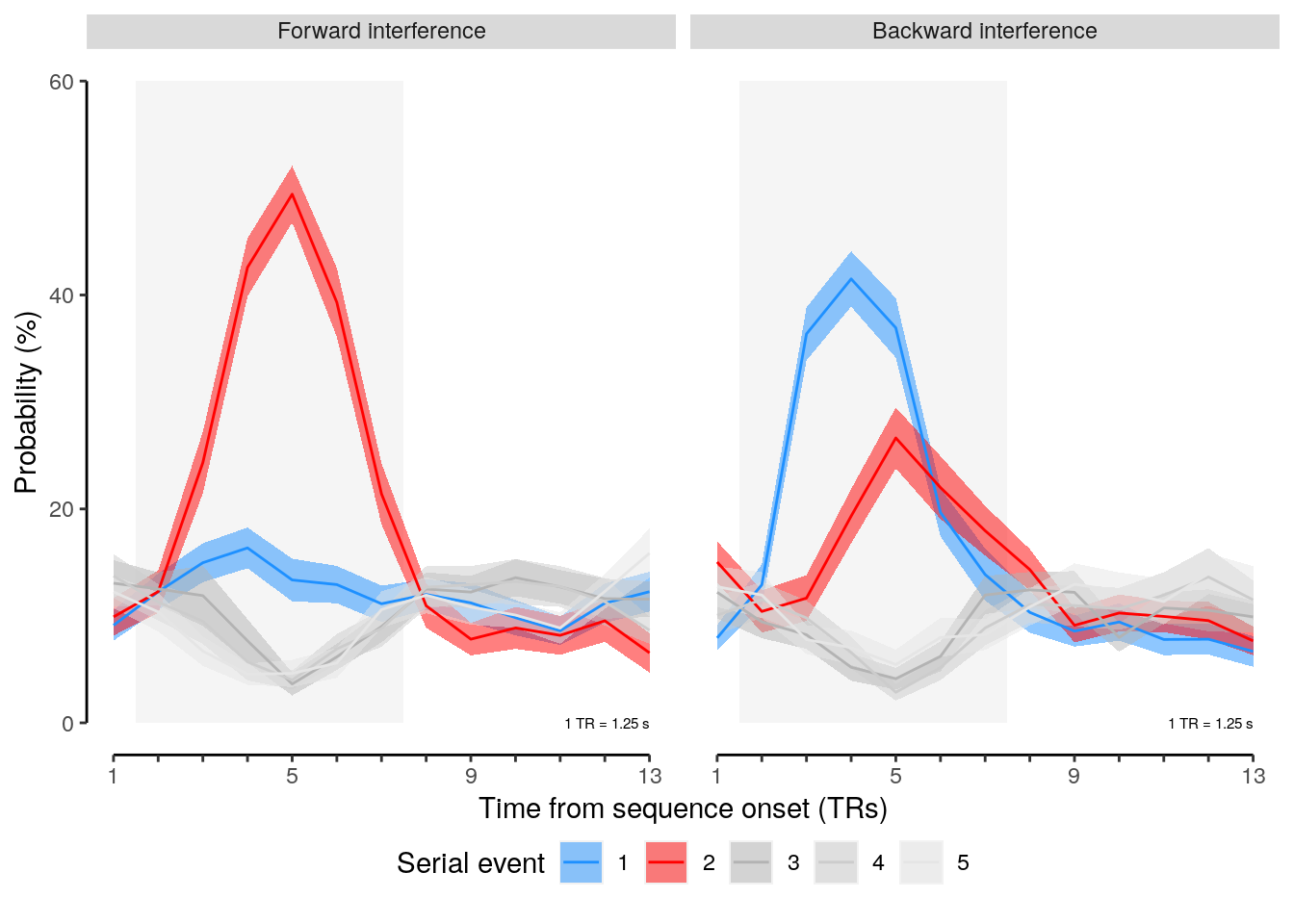
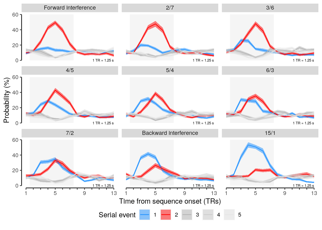
2.8.2.2 Source Data File Fig. 4a
subset(dt_pred_rep_timecourses, classification == "ovr") %>%
select(-classification, -num_sub) %>%
write.csv(., file = file.path(path_sourcedata, "source_data_figure_4a.csv"),
row.names = FALSE)2.8.3 Mean probabilities
2.8.3.1 Figure 4b
We calculate the mean decoding probabilities for each event:
# define the subset of selected TRs:
trs = seq(2, 7)
# calculate the mean probability for the event types across conditions:
dt_pred_rep_prob = dt_pred_rep %>%
# only consider the two extreme conditions (2 and 9):
filter(change %in% c(2, 9)) %>% verify(length(unique(change)) == 2) %>% setDT(.) %>%
# verify that the number of repetition trials per condition is correct:
verify(all(.[, by = .(classification, id, change), .(
num_trials = length(unique(trial))
)]$num_trials == 5)) %>%
# filter specific TRs:
filter(seq_tr %in% trs) %>%
transform(probability_z = scale(probability)) %>%
filter(classification == "ovr") %>% setDT(.)
# calculate the mean probability for each position label:
dt_pred_rep_mean_prob = dt_pred_rep_prob %>%
# calculate the mean probability for each position label on each trial:
.[, by = .(id, classification, trial, position_label), .(
num_events = .N,
probability = mean(probability * 100)
)] %>%
# verify that the number of events for each position label is correct:
verify(all(num_events %in% c(length(trs), length(trs) * 3))) %>%
# set the position label as factor and z-score the probability values:
mutate(position_label = as.factor(position_label)) %>%
transform(probability_z = scale(probability)) %>%
setorder(id, classification, trial, position_label)
# average the data for each position label across trials:
dt_pred_rep_mean_prob_plot = dt_pred_rep_mean_prob %>% setDT(.) %>%
.[, by = .(id, classification, position_label), .(
num_trials = .N,
probability = mean(probability)
)] %>% verify(all(num_trials == 10))# define linear mixed effects model with by-participant random intercepts:
lme_rep_mean_prob = lmer(probability ~ position_label + (1 + position_label|id),
data = subset(dt_pred_rep_mean_prob, classification == "ovr"), control = lcctrl)
summary(lme_rep_mean_prob)## Linear mixed model fit by REML. t-tests use Satterthwaite's method [
## lmerModLmerTest]
## Formula: probability ~ position_label + (1 + position_label | id)
## Data: subset(dt_pred_rep_mean_prob, classification == "ovr")
## Control: lcctrl
##
## REML criterion at convergence: 9002.9
##
## Scaled residuals:
## Min 1Q Median 3Q Max
## -1.6657 -0.6370 -0.1176 0.4832 4.0397
##
## Random effects:
## Groups Name Variance Std.Dev. Corr
## id (Intercept) 6.930 2.632
## position_label2 20.593 4.538 -0.94
## position_labelnone 5.728 2.393 -1.00 0.91
## Residual 242.541 15.574
## Number of obs: 1080, groups: id, 36
##
## Fixed effects:
## Estimate Std. Error df t value Pr(>|t|)
## (Intercept) 20.1857 0.9307 35.0264 21.688 < 2e-16 ***
## position_label2 4.5897 1.3855 35.2853 3.313 0.00214 **
## position_labelnone -12.4656 1.2274 85.1270 -10.156 2.45e-16 ***
## ---
## Signif. codes: 0 '***' 0.001 '**' 0.01 '*' 0.05 '.' 0.1 ' ' 1
##
## Correlation of Fixed Effects:
## (Intr) pstn_2
## positn_lbl2 -0.764
## postn_lblnn -0.743 0.558anova(lme_rep_mean_prob)## Type III Analysis of Variance Table with Satterthwaite's method
## Sum Sq Mean Sq NumDF DenDF F value Pr(>F)
## position_label 53424 26712 2 57.776 110.13 < 2.2e-16 ***
## ---
## Signif. codes: 0 '***' 0.001 '**' 0.01 '*' 0.05 '.' 0.1 ' ' 1emmeans_results = emmeans(lme_rep_mean_prob, list(pairwise ~ position_label))
print(emmeans_results)## $`emmeans of position_label`
## position_label emmean SE df lower.CL upper.CL
## 1 20.19 0.931 35 18.30 22.08
## 2 24.78 0.903 35 22.94 26.61
## none 7.72 0.822 35 6.05 9.39
##
## Degrees-of-freedom method: kenward-roger
## Confidence level used: 0.95
##
## $`pairwise differences of position_label`
## contrast estimate SE df t.ratio p.value
## 1 - 2 -4.59 1.39 35 -3.313 0.0060
## 1 - none 12.47 1.23 35 10.156 <.0001
## 2 - none 17.06 1.24 35 13.797 <.0001
##
## Degrees-of-freedom method: kenward-roger
## P value adjustment: tukey method for comparing a family of 3 estimatesemmeans_pvalues = round_pvalues(summary(emmeans_results[[2]])$p.value)dt_significance = data.table(
contrast = emmeans_results$contrast,
position_label = rep(c("1", "2", "none"), each = 2),
group = c(1.5, 2.0, 2.5),
probability = c(55, 75, 65),
pvalue = emmeans_pvalues
)fig_b = ggplot(data = subset(dt_pred_rep_mean_prob_plot, classification == "ovr"), aes(
x = as.factor(position_label), y = as.numeric(probability),
fill = as.factor(position_label))) +
geom_flat_violin(scale = "width", trim = FALSE, aes(color = NA),
position = position_nudge(x = 0.2, y = 0), alpha = 0.4) +
geom_point(stat = "summary", fun = "mean", color = "black", pch = 23, size = 3,
position = position_nudge(x = 0.125, y = 0)) +
geom_errorbar(stat = "summary", fun.data = "mean_se", width = 0.0,
position = position_nudge(x = 0.125, y = 0), color = "black") +
geom_boxplot(outlier.colour = "black", outlier.shape = NA, alpha = 0.5,
notch = FALSE, outlier.alpha = 1, width = 0.05, color = "black",
position = position_nudge(x = 0.25, y = 0)) +
geom_point(position = position_jitter(width = .05, height = 0, seed = 4),
pch = 21, alpha = 1, color = "black") +
xlab("Serial event") + ylab("Probability (%)") +
scale_fill_manual(name = "Serial event", values = colors) +
scale_color_manual(name = "Serial event", values = colors) +
#scale_y_continuous(labels = label_fill(seq(0, 100, 10), mod = 2), breaks = seq(0, 100, 10)) +
coord_capped_cart(left = "both", bottom = "both", ylim = c(0, 100)) +
theme(legend.position = "bottom", legend.direction = "horizontal",
legend.justification = "center", legend.margin = margin(0,0,0,0),
legend.box.margin = margin(t = -10, r = 0, b = 10, l = 0)) +
theme(panel.background = element_blank()) +
#theme(plot.margin = unit(c(t = 1, r = 1, b = 1, l = 1), "pt")) +
geom_line(data = dt_significance, aes(group = group),
linetype = "solid", position = position_nudge(x = 0.1, y = 0)) +
geom_text(data = dt_significance %>% distinct(group, probability, .keep_all = TRUE),
aes(x = group, y = probability + 1.5, label = pvalue), color = "black",
position = position_nudge(x = 0.125, y = 4), parse = FALSE) +
theme(axis.line.y = element_line(colour = "black"),
axis.line.x = element_line(colour = "white"),
panel.grid.major = element_blank(),
panel.grid.minor = element_blank(),
panel.border = element_blank(),
panel.background = element_blank(),
axis.text.x = element_blank(),
axis.title.x = element_blank(),
axis.ticks.x = element_line(colour = "white"))
fig_b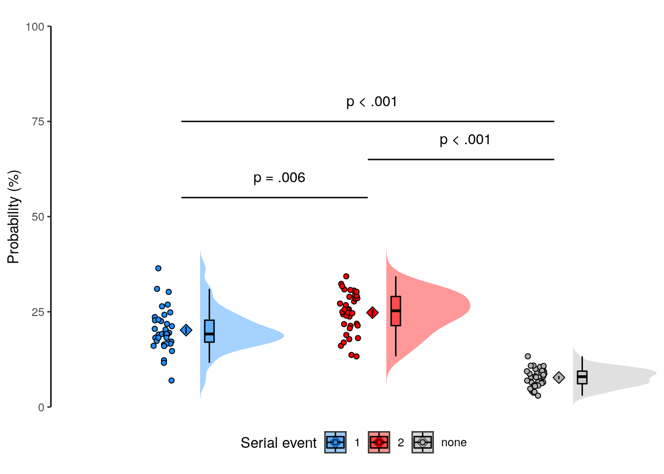
2.8.3.2 Source Data File Fig. 4b
subset(dt_pred_rep_mean_prob_plot, classification == "ovr") %>%
select(-classification, -num_trials) %>%
write.csv(., file = file.path(path_sourcedata, "source_data_figure_4b.csv"),
row.names = FALSE)2.8.3.3 Figure 4c
trs = seq(2, 7)
# calculate means for each participant:
dt_pred_rep_a2_sub = dt_pred_rep %>%
# only consider the two extreme conditions (2 and 9):
#filter(change %in% c(2,9)) %>%
filter(seq_tr %in% trs) %>%
# set the change variable to a factor:
transform(change = as.factor(change)) %>%
transform(position_label = as.factor(position_label)) %>% setDT(.) %>%
# check if the number of change conditions really only equals 2:
#verify(length(unique(change)) == 2) %>%
.[, by = .(id, classification, change, position_label), .(
probability = mean(probability * 100)
)] %>%
# standardize the probabilities:
#mutate(probability_z = scale(probability)) %>% setDT(.) %>%
setorder(id, classification, change, position_label) %>%
filter(classification == "ovr") %>% setDT(.)lme_data = dt_pred_rep_a2_sub %>% filter(classification == "ovr" & change %in% c(2,9))
lme_rep_prob_rep = lmer(probability ~ position_label * change + (1 + position_label + change|id),
data = lme_data, na.action = na.omit, control = lcctrl)
summary(lme_rep_prob_rep)## Linear mixed model fit by REML. t-tests use Satterthwaite's method [
## lmerModLmerTest]
## Formula: probability ~ position_label * change + (1 + position_label +
## change | id)
## Data: lme_data
## Control: lcctrl
##
## REML criterion at convergence: 1364.3
##
## Scaled residuals:
## Min 1Q Median 3Q Max
## -2.08370 -0.61552 -0.02366 0.55922 2.57687
##
## Random effects:
## Groups Name Variance Std.Dev. Corr
## id (Intercept) 16.3158 4.0393
## position_label2 42.2923 6.5033 -0.86
## position_labelnone 16.3072 4.0382 -0.98 0.74
## change9 0.9134 0.9557 0.34 0.18 -0.54
## Residual 26.6103 5.1585
## Number of obs: 216, groups: id, 36
##
## Fixed effects:
## Estimate Std. Error df t value Pr(>|t|)
## (Intercept) 13.499 1.092 54.859 12.362 < 2e-16 ***
## position_label2 18.052 1.629 64.902 11.083 < 2e-16 ***
## position_labelnone -5.748 1.390 93.815 -4.136 7.70e-05 ***
## change9 13.373 1.226 137.028 10.905 < 2e-16 ***
## position_label2:change9 -26.925 1.720 140.000 -15.658 < 2e-16 ***
## position_labelnone:change9 -13.436 1.720 140.000 -7.814 1.19e-12 ***
## ---
## Signif. codes: 0 '***' 0.001 '**' 0.01 '*' 0.05 '.' 0.1 ' ' 1
##
## Correlation of Fixed Effects:
## (Intr) pstn_2 pstn_l chang9 ps_2:9
## positn_lbl2 -0.770
## postn_lblnn -0.779 0.564
## change9 -0.524 0.385 0.400
## pstn_lbl2:9 0.394 -0.528 -0.309 -0.701
## pstn_lbln:9 0.394 -0.264 -0.619 -0.701 0.500anova(lme_rep_prob_rep)## Type III Analysis of Variance Table with Satterthwaite's method
## Sum Sq Mean Sq NumDF DenDF F value Pr(>F)
## position_label 7778.4 3889.2 2 41.642 146.1547 <2e-16 ***
## change 0.3 0.3 1 90.029 0.0126 0.9109
## position_label:change 6524.4 3262.2 2 140.000 122.5913 <2e-16 ***
## ---
## Signif. codes: 0 '***' 0.001 '**' 0.01 '*' 0.05 '.' 0.1 ' ' 1emmeans_results = emmeans(lme_rep_prob_rep, list(pairwise ~ position_label | change))
print(emmeans_results)## $`emmeans of position_label | change`
## change = 2:
## position_label emmean SE df lower.CL upper.CL
## 1 13.50 1.092 53.8 11.31 15.69
## 2 31.55 1.052 55.6 29.44 33.66
## none 7.75 0.872 68.8 6.01 9.49
##
## change = 9:
## position_label emmean SE df lower.CL upper.CL
## 1 26.87 1.137 52.0 24.59 29.15
## 2 18.00 1.126 52.4 15.74 20.26
## none 7.69 0.863 69.7 5.97 9.41
##
## Degrees-of-freedom method: kenward-roger
## Confidence level used: 0.95
##
## $`pairwise differences of position_label | change`
## change = 2:
## contrast estimate SE df t.ratio p.value
## 1 - 2 -18.05 1.63 62.6 -11.083 <.0001
## 1 - none 5.75 1.39 77.0 4.136 0.0003
## 2 - none 23.80 1.43 74.3 16.701 <.0001
##
## change = 9:
## contrast estimate SE df t.ratio p.value
## 1 - 2 8.87 1.63 62.6 5.447 <.0001
## 1 - none 19.18 1.39 77.0 13.804 <.0001
## 2 - none 10.31 1.43 74.3 7.236 <.0001
##
## Degrees-of-freedom method: kenward-roger
## P value adjustment: tukey method for comparing a family of 3 estimatesemmeans_summary = summary(emmeans_results[[2]])dt_significance = data.table(
change = rep(emmeans_summary$change, each = 2),
contrast = rep(emmeans_summary$contrast, each = 2),
pvalue = rep(round_pvalues(emmeans_summary$p.value), each = 2),
group = rep(c(1.5, 2.0, 2.5), each = 2),
position_label = c("1", "2", "1", "none", "2", "none"),
probability = rep(c(60, 80, 70), each = 2)
)dt_plot = dt_pred_rep_a2_sub %>% filter(classification == "ovr" & change %in% c(2,9))
fig_c = ggplot(data = dt_plot, aes(
x = as.factor(position_label), y = as.numeric(probability),
fill = as.factor(position_label))) +
geom_flat_violin(
scale = "width", trim = FALSE, aes(color = NA),
position = position_nudge(x = 0.25, y = 0), alpha = 0.4) +
geom_point(
stat = "summary", fun = "mean", color = "black", pch = 23, size = 3,
position = position_nudge(x = 0.15, y = 0)) +
geom_errorbar(
stat = "summary", fun.data = "mean_se", width = 0.0,
position = position_nudge(x = 0.15, y = 0), color = "black") +
geom_boxplot(
outlier.colour = "black", outlier.shape = NA, outlier.size = 50,
notch = FALSE, outlier.alpha = 1, width = 0.05, color = "black",
position = position_nudge(x = 0.35, y = 0), alpha = 0.5) +
geom_point(
position = position_jitter(width = .05, height = 0, seed = 4),
pch = 21, alpha = 1) +
facet_wrap(~ as.factor(change), labeller = as_labeller(facet_labels_new)) +
xlab("Serial event") + ylab("Probability (%)") +
scale_fill_manual(name = "Serial event", values = colors) +
scale_color_manual(name = "Serial event", values = colors) +
#scale_y_continuous(labels = label_fill(seq(0, 100, 10), mod = 2), breaks = seq(0, 100, 10)) +
coord_capped_cart(left = "both", bottom = "both", ylim = c(0, 100), expand = TRUE) +
theme(legend.position = "bottom", legend.direction = "horizontal",
legend.justification = "center", legend.margin = margin(0,0,0,0),
legend.box.margin = margin(t = -10, r = 0, b = 10, l = 0)) +
theme(panel.background = element_blank()) +
theme(strip.text.x = element_text(margin = margin(b = 3, t = 2))) +
theme(axis.title.x = element_blank(), axis.text.x = element_blank(),
axis.ticks.x = element_blank(), axis.line.x = element_blank()) +
#theme(plot.margin = unit(c(t = 1, r = 1, b = 1, l = 1), "pt")) +
geom_line(data = dt_significance, aes(group = group, x = position_label, y = probability),
linetype = "solid", position = position_nudge(x = 0.1, y = 0)) +
geom_text(data = dt_significance %>% distinct(group, change, probability, .keep_all = TRUE),
aes(x = group, y = probability + 1, label = pvalue), color = "black",
position = position_nudge(x = 0.1, y = 4), parse = FALSE) +
theme(axis.line.y = element_line(colour = "black"),
axis.line.x = element_line(colour = "white"),
panel.grid.major = element_blank(),
panel.grid.minor = element_blank(),
panel.border = element_blank(),
panel.background = element_blank(),
axis.text.x = element_blank(),
axis.title.x = element_blank(),
axis.ticks.x = element_line(colour = "white"))
fig_c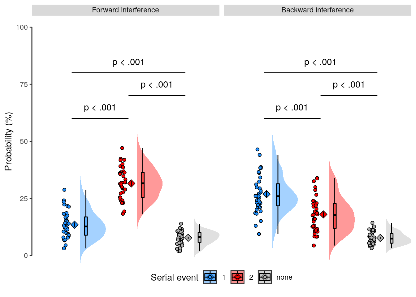
2.8.3.4 Source Data File Fig. 4c
subset(dt_pred_rep_a2_sub, classification == "ovr") %>%
select(-classification) %>%
write.csv(., file = file.path(path_sourcedata, "source_data_figure_4c.csv"),
row.names = FALSE)2.8.3.5 Figure S8
# select specific trs:
trs = seq(2, 7)
dt_pred_rep_all_reps_sub = dt_pred_rep %>%
# filter out the extremely long condition (with 16 items):
filter(occurence != 15) %>% setDT(.) %>%
# filter for specific trs:
filter(seq_tr %in% trs) %>% setDT(.) %>%
# transform the main variables of interest:
transform(
occurence = as.numeric(occurence),
position_label = as.factor(position_label),
probability = probability * 100
) %>% setDT(.) %>%
# calculate the mean probability for each serial event item (first, second, other)
# separately depending on the number of indiviual repetitions
.[, by = .(id, classification, occurence, position_label), .(
probability = mean(probability)
)] %>%
setorder(., classification, id, occurence, position_label)
dt_pred_rep_all_reps_mean = dt_pred_rep_all_reps_sub %>%
# average across participants and calculate the standard error of the mean:
. [, by = .(classification, occurence, position_label), {
list(
mean_probability = mean(probability),
num_subs = .N,
sem_upper = mean(probability) + (sd(probability)/sqrt(.N)),
sem_lower = mean(probability) - (sd(probability)/sqrt(.N))
)}] %>%
verify(all(num_subs == 36)) %>%
setorder(., classification, occurence, position_label)Are the short repetitions of event 1 and event 2 different from noise:
LME model including all three event types:
# model including all three event types:
lme_pred_rep_all_reps = lmer(probability ~ position_label * occurence + (1 + position_label + occurence|id),
data = subset(dt_pred_rep_all_reps_sub, classification == "ovr" & occurence != 15),
na.action = na.omit, control = lcctrl)
summary(lme_pred_rep_all_reps)## Linear mixed model fit by REML. t-tests use Satterthwaite's method [
## lmerModLmerTest]
## Formula: probability ~ position_label * occurence + (1 + position_label +
## occurence | id)
## Data:
## subset(dt_pred_rep_all_reps_sub, classification == "ovr" & occurence !=
## 15)
## Control: lcctrl
##
## REML criterion at convergence: 5592
##
## Scaled residuals:
## Min 1Q Median 3Q Max
## -3.2610 -0.5744 -0.0611 0.5061 3.6198
##
## Random effects:
## Groups Name Variance Std.Dev. Corr
## id (Intercept) 3.07985 1.7550
## position_label2 7.56801 2.7510 -0.28
## position_labelnone 4.41464 2.1011 -0.62 -0.04
## occurence 0.06141 0.2478 0.05 0.32 -0.81
## Residual 34.75199 5.8951
## Number of obs: 864, groups: id, 36
##
## Fixed effects:
## Estimate Std. Error df t value Pr(>|t|)
## (Intercept) 11.58826 0.81954 160.93054 14.140 < 2e-16
## position_label2 4.65762 1.17576 274.88239 3.961 9.5e-05
## position_labelnone -3.87294 1.13790 389.16818 -3.404 0.000734
## occurence 1.90219 0.15713 313.08078 12.106 < 2e-16
## position_label2:occurence 0.08274 0.21440 752.99954 0.386 0.699656
## position_labelnone:occurence -1.86040 0.21440 752.99953 -8.677 < 2e-16
##
## (Intercept) ***
## position_label2 ***
## position_labelnone ***
## occurence ***
## position_label2:occurence
## position_labelnone:occurence ***
## ---
## Signif. codes: 0 '***' 0.001 '**' 0.01 '*' 0.05 '.' 0.1 ' ' 1
##
## Correlation of Fixed Effects:
## (Intr) pstn_2 pstn_l occrnc pst_2:
## positn_lbl2 -0.647
## postn_lblnn -0.697 0.433
## occurence -0.798 0.592 0.513
## pstn_lbl2:c 0.589 -0.821 -0.424 -0.682
## pstn_lblnn: 0.589 -0.410 -0.848 -0.682 0.500anova(lme_pred_rep_all_reps)## Type III Analysis of Variance Table with Satterthwaite's method
## Sum Sq Mean Sq NumDF DenDF F value Pr(>F)
## position_label 1667.4 833.7 2 278.97 23.989 2.435e-10 ***
## occurence 6363.2 6363.2 1 58.73 183.102 < 2.2e-16 ***
## position_label:occurence 3650.8 1825.4 2 753.00 52.527 < 2.2e-16 ***
## ---
## Signif. codes: 0 '***' 0.001 '**' 0.01 '*' 0.05 '.' 0.1 ' ' 1LME model excluding out-of-sequence events:
lme_pred_rep_all_reps_reduced = lmer(probability ~ position_label * occurence + (1 + position_label + occurence|id),
data = subset(dt_pred_rep_all_reps_sub, classification == "ovr" & occurence != 15 & position_label != "none"),
na.action = na.omit, control = lcctrl)## Warning: Model failed to converge with 1 negative eigenvalue: -6.7e+00summary(lme_pred_rep_all_reps_reduced)## Linear mixed model fit by REML. t-tests use Satterthwaite's method [
## lmerModLmerTest]
## Formula: probability ~ position_label * occurence + (1 + position_label +
## occurence | id)
## Data:
## subset(dt_pred_rep_all_reps_sub, classification == "ovr" & occurence !=
## 15 & position_label != "none")
## Control: lcctrl
##
## REML criterion at convergence: 3927.2
##
## Scaled residuals:
## Min 1Q Median 3Q Max
## -2.83205 -0.66198 -0.07749 0.63366 3.02136
##
## Random effects:
## Groups Name Variance Std.Dev. Corr
## id (Intercept) 0.000 0.0000
## position_label2 4.212 2.0523 NaN
## occurence 0.133 0.3647 NaN 0.38
## Residual 49.631 7.0450
## Number of obs: 576, groups: id, 36
##
## Fixed effects:
## Estimate Std. Error df t value Pr(>|t|)
## (Intercept) 11.58826 0.91490 501.89714 12.666 < 2e-16 ***
## position_label2 4.65762 1.33831 350.19281 3.480 0.000564 ***
## occurence 1.90219 0.19110 298.33537 9.954 < 2e-16 ***
## position_label2:occurence 0.08274 0.25622 501.89714 0.323 0.746875
## ---
## Signif. codes: 0 '***' 0.001 '**' 0.01 '*' 0.05 '.' 0.1 ' ' 1
##
## Correlation of Fixed Effects:
## (Intr) pstn_2 occrnc
## positn_lbl2 -0.684
## occurence -0.845 0.609
## pstn_lbl2:c 0.630 -0.862 -0.670anova(lme_pred_rep_all_reps_reduced)## Type III Analysis of Variance Table with Satterthwaite's method
## Sum Sq Mean Sq NumDF DenDF F value Pr(>F)
## position_label 601.1 601.1 1 350.19 12.1119 0.0005643 ***
## occurence 9323.8 9323.8 1 125.87 187.8611 < 2.2e-16 ***
## position_label:occurence 5.2 5.2 1 501.90 0.1043 0.7468748
## ---
## Signif. codes: 0 '***' 0.001 '**' 0.01 '*' 0.05 '.' 0.1 ' ' 1dt_pred_rep_all_reps_stats = dt_pred_rep_all_reps_sub %>%
filter(occurence %in% c(8)) %>% setDT(.) %>%
transform(position_label = paste0("pos_", position_label)) %>%
spread(key = position_label, value = probability, drop = FALSE) %>%
filter(classification == "ovr")
# some ugly code to perform three t-tests:
summary(dt_pred_rep_all_reps_stats$pos_2); round(sd(dt_pred_rep_all_reps_stats$pos_2), 2)## Min. 1st Qu. Median Mean 3rd Qu. Max.
## 18.27 25.46 31.63 31.55 36.37 47.05## [1] 6.94summary(dt_pred_rep_all_reps_stats$pos_1); round(sd(dt_pred_rep_all_reps_stats$pos_1), 2)## Min. 1st Qu. Median Mean 3rd Qu. Max.
## 9.432 21.742 25.970 26.872 31.418 46.455## [1] 8.34summary(dt_pred_rep_all_reps_stats$pos_none); round(sd(dt_pred_rep_all_reps_stats$pos_none), 2)## Min. 1st Qu. Median Mean 3rd Qu. Max.
## 3.195 5.395 7.396 7.689 9.562 14.290## [1] 2.69# perform separate t-tests
test1 = t.test(dt_pred_rep_all_reps_stats$pos_2, dt_pred_rep_all_reps_stats$pos_1,
paired = TRUE, alternative = "two.sided")
test2 = t.test(dt_pred_rep_all_reps_stats$pos_2, dt_pred_rep_all_reps_stats$pos_none,
paired = TRUE, alternative = "two.sided")
test3 = t.test(dt_pred_rep_all_reps_stats$pos_1, dt_pred_rep_all_reps_stats$pos_none,
paired = TRUE, alternative = "two.sided")
test1; test2; test3##
## Paired t-test
##
## data: dt_pred_rep_all_reps_stats$pos_2 and dt_pred_rep_all_reps_stats$pos_1
## t = 2.5877, df = 35, p-value = 0.01397
## alternative hypothesis: true difference in means is not equal to 0
## 95 percent confidence interval:
## 1.008362 8.350423
## sample estimates:
## mean of the differences
## 4.679393##
## Paired t-test
##
## data: dt_pred_rep_all_reps_stats$pos_2 and dt_pred_rep_all_reps_stats$pos_none
## t = 18.964, df = 35, p-value < 2.2e-16
## alternative hypothesis: true difference in means is not equal to 0
## 95 percent confidence interval:
## 21.30830 26.41741
## sample estimates:
## mean of the differences
## 23.86285##
## Paired t-test
##
## data: dt_pred_rep_all_reps_stats$pos_1 and dt_pred_rep_all_reps_stats$pos_none
## t = 12.518, df = 35, p-value = 1.75e-14
## alternative hypothesis: true difference in means is not equal to 0
## 95 percent confidence interval:
## 16.07247 22.29445
## sample estimates:
## mean of the differences
## 19.18346# correct for multiple comparisons
p.adjust(c(test1$p.value, test2$p.value, test3$p.value), method = "bonferroni", n = 6)## [1] 8.383045e-02 3.250184e-19 1.049727e-13fig_d = ggplot(data = subset(dt_pred_rep_all_reps_mean, classification == "ovr"), aes(
x = as.factor(occurence), y = as.numeric(mean_probability),
group = as.factor(position_label), color = as.factor(position_label))) +
geom_ribbon(aes(ymin = sem_lower, ymax = sem_upper,
fill = as.factor(position_label)), alpha = 0.5) +
geom_line(size = 0.7, mapping = aes(color = as.factor(position_label))) +
xlab("Number of item repetitions") +
ylab("Probability (in %)") +
scale_fill_manual(name = "Serial event", values = colors) +
scale_color_manual(name = "Serial event", values = colors) +
scale_y_continuous(labels = label_fill(seq(0, 100, 10), mod = 2), breaks = seq(0, 100, 10)) +
coord_capped_cart(left = "both", bottom = "both", expand = TRUE, ylim = c(0,40)) +
theme(legend.position = "right", legend.direction = "vertical") +
guides(color = guide_legend(ncol = 1)) +
theme(legend.position = "right", legend.direction = "vertical",
legend.justification = "center", legend.margin = margin(0,0,0,0),
legend.box.margin = margin(t = 0, r = , b = 0, l = -20)) +
theme(panel.background = element_blank()) +
theme(plot.margin = unit(c(t = 1, r = 1, b = 1, l = 1), "pt")) +
theme(axis.line = element_line(colour = "black"),
panel.grid.major = element_blank(),
panel.grid.minor = element_blank(),
panel.border = element_blank(),
panel.background = element_blank())
fig_d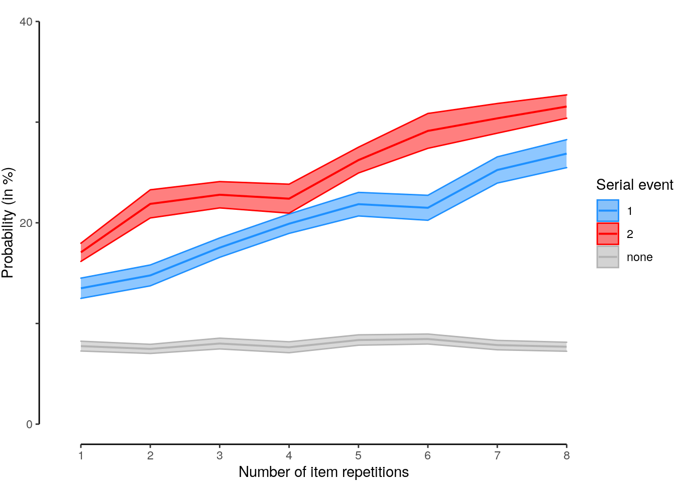
2.8.3.6 Source Data File Fig. S8
subset(dt_pred_rep_all_reps_mean, classification == "ovr") %>%
select(-classification, -num_subs) %>%
write.csv(., file = file.path(path_sourcedata, "source_data_figure_s8.csv"),
row.names = FALSE)2.8.4 Step-sizes
Are there more within sequence items in the classifier predictions? To this end, we check if serial events 1 and 2 (of 2) are decoded more often than other (out-of-sequence) serial events in the repetition trials.
# define the number of TRs per trial (used below):
select_trs = seq(2, 7)
dt_pred_rep_count = dt_pred_rep %>%
# get the position with the highest probability:
.[, by = .(classification, id, trial, change, seq_tr), ":=" (
num_events = .N,
position_max_prob = as.numeric(probability == max(probability))
)] %>%
# check if the data consisted of 5 trials per TR:
verify(num_events == 5) %>%
# check if there is only one event with the maximum probability:
verify(.[, by = .(classification, id, trial, change, seq_tr), .(
num_max_events = sum(position_max_prob)
)]$num_max_events == 1) %>%
# get the position with the highest probability:
filter(position_max_prob == 1) %>%
setDT(.) %>%
# WARNING: HERE WE FILTER OUT SPECIFIC TRIALS SET ABOVE:
filter(seq_tr %in% select_trs) %>%
setDT(.) %>%
# calculate the absolute and relative occurrence of each maximum position:
.[, by = .(classification, id, change, trial, position), .(
count_num = .N / length(select_trs),
freq = .N
)] %>%
# complete missing positions with zeros:
complete(nesting(classification, id, change, trial),
nesting(position), fill = list(count_num = 0, freq = 0)) %>%
# create a new variable containing the type by copying the max position:
mutate(type = position) %>%
transform(type = ifelse(type %in% c(1,2), type, "none")) %>% setDT(.) %>%
# sort the data table
setorder(., classification, id, change, trial, position, type) %>%
# check if the sum of frequencies matches the number of trs:
verify(.[, by = .(classification, id, change, trial), .(
sum_freq = sum(freq)
)]$sum_freq == length(select_trs)) %>%
# average relative proportion of each position across trials per change:
setDT(.) %>% .[, by = .(classification, id, change, type), .(
mean_count = mean(count_num) * 100,
sum_freq = sum(freq),
num_trials = .N
)] %>%
#check if the data consisted of 5 trials per TR:
verify(num_trials %in% c(5, 15)) %>%
# change variable types for mixed effects models:
transform(change = as.factor(change)) %>%
transform(type = as.factor(type)) %>%
#mutate(mean_count_z = scale(mean_count, center = TRUE, scale = FALSE)) %>% setDT(.) %>%
# create a new variable:
.[type == "1", ":=" (is_first = 1, is_second = 0)] %>%
.[type == "2", ":=" (is_first = 0, is_second = 1)] %>%
.[type == "none", ":=" (is_first = 0, is_second = 0)] %>%
transform(is_first = as.numeric(is_first)) %>%
transform(is_second = as.numeric(is_second))dt_pred_rep_count_mean = dt_pred_rep_count %>%
# average the number of counts across participants:
setDT(.) %>%
.[, by = .(classification, change, type), .(
mean_count = mean(mean_count),
sd_count = sd(mean_count),
num_subs = .N,
sem_upper = mean(mean_count) + (sd(mean_count)/sqrt(.N)),
sem_lower = mean(mean_count) - (sd(mean_count)/sqrt(.N))
)] %>%
# check if the number of data points (here, participants) is correct:
verify(num_subs == 36) %>%
#verify(.[, by = .(classification, change), .(
# mean_count = sum(mean_count)
#)]$mean_count == 100) %>%
# order the data table:
setorder(., classification, change, type)lme_rep_count = lmer(mean_count ~ type * change + (1 + type + change|id),
data = subset(dt_pred_rep_count, classification == "ovr" & change %in% c(2,9)),
na.action = na.omit, control = lcctrl)
summary(lme_rep_count)## Linear mixed model fit by REML. t-tests use Satterthwaite's method [
## lmerModLmerTest]
## Formula: mean_count ~ type * change + (1 + type + change | id)
## Data: subset(dt_pred_rep_count, classification == "ovr" & change %in%
## c(2, 9))
## Control: lcctrl
##
## REML criterion at convergence: 1481.9
##
## Scaled residuals:
## Min 1Q Median 3Q Max
## -2.31498 -0.56768 0.04092 0.53526 2.53048
##
## Random effects:
## Groups Name Variance Std.Dev. Corr
## id (Intercept) 19.835 4.4536
## type2 92.142 9.5991 -0.79
## typenone 27.993 5.2908 -0.97 0.61
## change9 0.637 0.7981 0.32 -0.84 -0.07
## Residual 46.779 6.8395
## Number of obs: 216, groups: id, 36
##
## Fixed effects:
## Estimate Std. Error df t value Pr(>|t|)
## (Intercept) 19.352 1.360 67.130 14.226 < 2e-16 ***
## type2 24.537 2.271 60.844 10.804 8.82e-16 ***
## typenone -7.099 1.837 91.869 -3.863 0.000208 ***
## change9 16.759 1.618 140.223 10.361 < 2e-16 ***
## type2:change9 -34.907 2.280 140.000 -15.311 < 2e-16 ***
## typenone:change9 -16.296 2.280 140.000 -7.148 4.45e-11 ***
## ---
## Signif. codes: 0 '***' 0.001 '**' 0.01 '*' 0.05 '.' 0.1 ' ' 1
##
## Correlation of Fixed Effects:
## (Intr) type2 typenn chang9 typ2:9
## type2 -0.723
## typenone -0.773 0.516
## change9 -0.576 0.305 0.434
## type2:chng9 0.419 -0.502 -0.310 -0.705
## typnn:chng9 0.419 -0.251 -0.620 -0.705 0.500anova(lme_rep_count)## Type III Analysis of Variance Table with Satterthwaite's method
## Sum Sq Mean Sq NumDF DenDF F value Pr(>F)
## type 10785 5392.5 2 38.108 115.2755 <2e-16 ***
## change 5 5.0 1 125.584 0.1078 0.7433
## type:change 10983 5491.4 2 140.000 117.3905 <2e-16 ***
## ---
## Signif. codes: 0 '***' 0.001 '**' 0.01 '*' 0.05 '.' 0.1 ' ' 1emmeans_results = emmeans(lme_rep_count, list(pairwise ~ type | change))
emmeans_summary = summary(emmeans_results[[2]])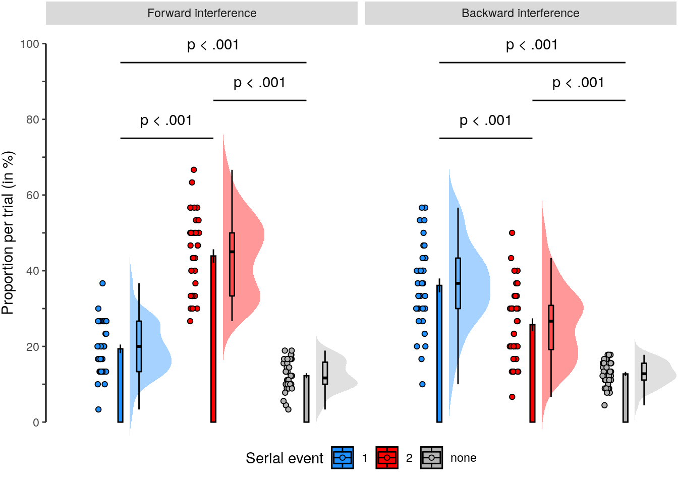
Test for significance
Test 1: Using a paired t-test, we test how well we are able to decode a single briefly presented item in a 32 ms sequence compared to items that were not presented, when the item (first event) is followed by a statistical representation that could mask the item (change = 2 condition).
Test 2: Using a paired t-test, we then test how well we are able to decode a single briefly presented item in a 32 ms sequence compared to items that were not presented, when the item (last event) is preceded by a statistical signal (change = 9 condition).
2.8.5 Transitions
We analyzed if there more within sequence transitions than transitions to out-of-sequence elements:
transition_type <- function(head, tail){
if (head == 1 & tail == 2){
transition_type = "forward"
} else if (head == 2 & tail == 1) {
transition_type = "backward"
} else if (head == 1 & tail == 1) {
transition_type = "repetition 1"
} else if (head == 2 & tail == 2) {
transition_type = "repetition 2"
#} else if(head == tail) {
# transition_type = "repetition"
} else if (head %in% c(1,2) & tail > 2) {
transition_type = "outwards"
} else if (head > 2 & tail %in% c(1,2)) {
transition_type = "inwards"
} else if (head > 2 & tail > 2 & head != tail) {
transition_type = "outside"
} else if (head > 2 & tail > 2 & head == tail) {
transition_type = "repetition out"
} else {
transition_type = "ERROR!"
}
return(transition_type)
}2.8.5.1 Figure 4e
trs = seq(2, 7)
# define the number of transitions, which is the number of TRs - 1
num_transitions = length(trs) - 1
# calculate the transitions between decoded repetition trial elements
dt_pred_rep_step = dt_pred_rep %>%
# filter for specific trs in a selected time window:
filter(seq_tr %in% trs) %>% setDT(.) %>%
# for each classification, id, trial, get position with highest probability:
.[, by = .(classification, id, trial, change, seq_tr), .(
num_trials = .N,
position_max = position[which.max(probability)]
)] %>%
# check if the data consisted of 5 trials per TR:
verify(num_trials == 5) %>%
# get the head and tail of the maximum positions (sequence shifted by 1):
# head = tr 1 to n-1 and tail = tr 2 to n:
.[, by = .(classification, id, trial, change), .(
n = .N,
head = head(position_max, -1),
tail = tail(position_max, -1)
)] %>%
# get the number of each unique combination of consecutive positions indices:
.[, .N, .(classification, id, trial, change, head, tail)] %>%
# complete all missing pairings with 0s for each trial:
complete(nesting(classification, id, trial, change), nesting(head, tail),
fill = list(N = 0)) %>% setDT(.) %>%
# check if the number of true transitions matching the expected number:
verify(.[, by = .(classification, id, trial, change), .(
sum_of_n = sum(N)
)]$sum_of_n == num_transitions) %>%
# set the order: sort by classification, participant, trial and positions:
setorder(classification, id, trial, change, head, tail) %>%
# define the transition type for every transition:
mutate(step_type = mapply(transition_type, head, tail)) %>%
# calculate the relative proportion per trial across TRs for each transition
mutate(proportion = N/num_transitions) %>% setDT(.) %>%
# check if any step type is not properly assigned:
verify(all(!is.na(step_type))) %>% setDT(.)
dt_pred_rep_step_version1 = dt_pred_rep_step %>%
# average the proportion of transitions across trials:
.[, by = .(classification, id, change, step_type), .(
mean_proportion = mean(proportion) * 100
)]
dt_pred_rep_step_version2 = dt_pred_rep_step %>%
# sum up the number of transitions for each transition type:
.[, by = .(classification, id, trial, change, step_type), .(
num = sum(N)
)] %>%
# check if the number of true transitions matching the expected number per trial:
#verify(.[, by = .(classification, id, trial, change), .(
# num_transitions = sum(num)
#)]$num_transitions == num_transitions) %>%
# calculate the proportion per trial across TRs for each transition
mutate(proportion = num/num_transitions) %>% setDT(.) %>%
# average the proportion of transitions across trials:
.[, by = .(classification, id, change, step_type), .(
mean_num = mean(num),
mean_proportion = mean(proportion) * 100
)]
dt_pred_rep_step_mean = dt_pred_rep_step_version1 %>%
# average across participants and compute the standard error:
.[, by = .(classification, change, step_type), .(
mean_proportion = mean(mean_proportion),
num_subs = .N,
sem_upper = mean(mean_proportion) + (sd(mean_proportion)/sqrt(.N)),
sem_lower = mean(mean_proportion) - (sd(mean_proportion)/sqrt(.N))
)] %>%
verify(all(num_subs == 36)) %>%
setorder(classification, change, step_type) %>%
filter(classification == "ovr")plot_rep_trans_mat = function(dt){
ggplot(data = dt, mapping = aes(
x = as.factor(head), y = fct_rev(as_factor(tail)),
size = mean_proportion, fill = step_type)) +
geom_point(aes(size = mean_proportion, fill = step_type), pch = 21, color = "black") +
coord_capped_cart(left = "both", bottom = "both", expand = TRUE) +
xlab("Decoded event at t") +
ylab("Decoded event at t + 1") +
facet_wrap(~ as.factor(change), labeller = as_labeller(facet_labels_new)) +
scale_size(range = c(1, 15), name = "Proportion per trial (in %)",
guide = guide_legend(
title.position = "top", direction = "horizontal",
nrow = 1,
order = 2)) +
scale_fill_manual(name = "Transition type",
values = c(colors, "white", "white", "white"),
guide = guide_legend(ncol = 2)) +
theme(strip.text.x = element_text(margin = margin(b = 3, t = 2))) +
scale_y_discrete(limits = rev(levels(~tail))) +
theme(axis.line = element_line(colour = "black"),
panel.grid.major = element_blank(),
panel.grid.minor = element_blank(),
panel.border = element_blank(),
panel.background = element_blank()) +
# remove background of legend keys:
theme(legend.key = element_blank()) +
theme(legend.background = element_blank())
# add annotation
#annotate("segment", x = 0, xend = 6, y = 6, yend = 0,
# colour = "white", size = 10, alpha = 0.8) +
#annotate(geom = "text", x = 3, y = 3, angle = 360 - 45, hjust = 0.5,
# label = "Repetitions of the same decoded event",
# color = "gray")
}dt_pred_rep_step_trans = dt_pred_rep_step %>%
.[, by = .(classification, change, head, tail, step_type), .(
num_data = .N,
mean_proportion = mean(proportion) * 100
)] %>%
# check if averaged is number of participants times number of trials
verify(all(num_data == 36 * 5)) %>%
# create new variable containing the the averaged number as a label:
mutate(mean_num_label = as.character(sub('^(-)?0[.]', '\\1.', round(mean_proportion, 2)))) %>%
# remove all repetition transitions:
mutate(step_type = ifelse(stringr::str_detect(step_type, "repetition"), "repetition", step_type)) %>%
setDT(.)fig_trans_mat = plot_rep_trans_mat(
dt = subset(dt_pred_rep_step_trans, classification == "ovr" & change %in% c(2,9)))
fig_trans_mat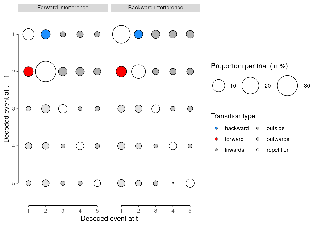
2.8.5.2 Source Data File Fig. 4e
subset(dt_pred_rep_step_trans, classification == "ovr" & change %in% c(2,9)) %>%
select(-classification, -num_data) %>%
write.csv(., file = file.path(path_sourcedata, "source_data_figure_4e.csv"),
row.names = FALSE)2.8.5.3 Figure 4d
plot_rep_trans <- function(dt){
ggplot(
data = dt, aes(x = as.factor(step_type), y = as.numeric(mean_proportion),
fill = as.factor(step_type))) +
geom_bar(stat = "summary", fun = "mean",
aes(fill = as.factor(step_type)),
color = "black",
position = position_dodge()) +
geom_point(position = position_jitter(width = .2, height = 0, seed = 4),
pch = 21, alpha = 0.5, color = "black") +
geom_errorbar(stat = "summary", fun.data = "mean_se", width = 0,
position = position_dodge(.9), color = "black") +
facet_wrap(~ as.factor(change), labeller = as_labeller(facet_labels_new)) +
xlab("Serial event") +
#xlab(expression(paste("Time-point of change to ", 2^nd, " serial event"))) +
ylab("Proportion per trial (%)") +
coord_capped_cart(left = "both", bottom = "both", expand = TRUE, ylim = c(0,10)) +
scale_fill_manual(name = "Transition", values = c(colors, "lightblue", "lightcoral", "darkgray")) +
theme(strip.text.x = element_text(margin = margin(b = 3, t = 2))) +
#scale_x_discrete(labels = as_labeller(facet_labels_new)) +
#theme(legend.position = "right", legend.direction = "vertical", legend.justification = "center") +
theme(legend.position = "bottom", legend.direction = "horizontal",
legend.justification = "center", legend.margin = margin(t = 0, r = 0, b = 0, l = 0),
legend.box.margin = margin(t = -10, r = 0, b = 10, l = 0)) +
guides(fill = guide_legend(nrow = 2, title.position = "top", title.hjust = 0.5)) +
theme(panel.background = element_blank()) +
#theme(plot.margin = unit(c(t = 1, r = 1, b = 1, l = 1), "pt")) +
theme(axis.line.y = element_line(colour = "black"),
axis.line.x = element_line(colour = "white"),
panel.grid.major = element_blank(),
panel.grid.minor = element_blank(),
panel.border = element_blank(),
panel.background = element_blank(),
axis.text.x = element_blank(),
axis.title.x = element_blank(),
axis.ticks.x = element_line(colour = "white"))
}
# & change %in% c(2,9)
fig_trans_prop = plot_rep_trans(dt = subset(
dt_pred_rep_step_version1, classification == "ovr" & change %in% c(2,9) &
step_type != "repetition 1" & step_type != "repetition 2" & step_type != "repetition out"
))
fig_trans_prop
2.8.5.4 Source Data File Fig. 4d
subset(
dt_pred_rep_step_version1, classification == "ovr" & change %in% c(2,9) &
step_type != "repetition 1" & step_type != "repetition 2" & step_type != "repetition out"
) %>%
select(-classification) %>%
write.csv(., file = file.path(path_sourcedata, "source_data_figure_4d.csv"),
row.names = FALSE)We compare the average proportion of forward transitions with the average proportion of outwards steps in the change = 2 condition. We also compare the average proportion of forward transitions with the average number of within out-of-sequence transitions:
dt_pred_rep_trans_test = dt_pred_rep_step_version1 %>%
filter(step_type %in% c("forward", "outwards", "outside") & change == 9) %>%
spread(key = step_type, value = mean_proportion, drop = TRUE) %>% setDT(.) %>%
.[, by = .(classification), {
ttest_outwards = t.test(x = forward, y = outwards, paired = TRUE);
ttest_outside = t.test(x = forward, y = outside, paired = TRUE);
list(mean_forward = round(mean(forward), 2),
mean_outwards = round(mean(outwards), 2),
mean_outside = round(mean(outside), 2),
df = ttest_outwards$parameter,
ttest_outwards_pvalue = p.adjust(ttest_outwards$p.value,
method = "bonferroni", n = 4),
ttest_outwards_tvalue = round(ttest_outwards$statistic, 2),
ttest_outside_pvalue = p.adjust(ttest_outside$p.value,
method = "bonferroni", n = 4),
ttest_outside_tvalue = round(ttest_outside$statistic, 2),
num_subs = .N)
}] %>%
verify(all(num_subs == 36)) %>%
filter(classification == "ovr")
dt_pred_rep_trans_test## classification mean_forward mean_outwards mean_outside df
## 1: ovr 7.22 2.67 1.06 35
## ttest_outwards_pvalue ttest_outwards_tvalue ttest_outside_pvalue
## 1: 4.17355e-05 5.14 7.054921e-08
## ttest_outside_tvalue num_subs
## 1: 7.26 362.8.6 Figure 4
plot_grid(plot_grid(fig_a, fig_b, labels = c("a", "b")),
#plot_grid(fig_c, fig_d, labels = c("c", "d")),
plot_grid(fig_c, fig_trans_prop, labels = c("c", "d")),
plot_grid(fig_trans_mat, labels = c("e")),
ncol = 1, label_fontface = "bold")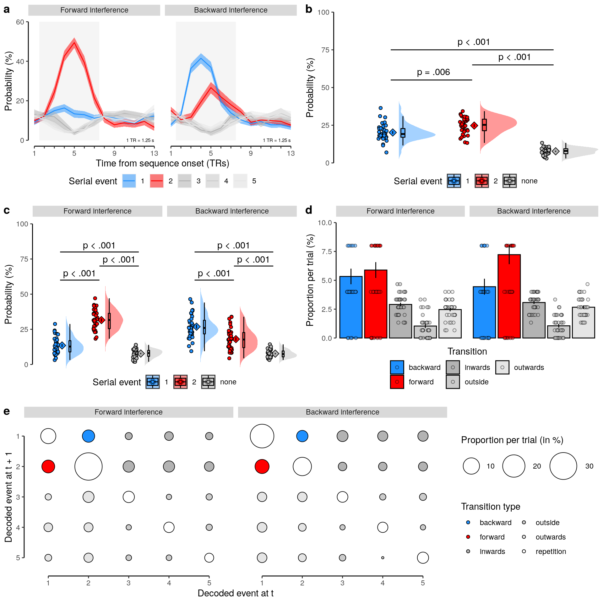
ggsave(filename = "wittkuhn_schuck_figure_4.pdf",
plot = last_plot(), device = cairo_pdf, path = path_figures, scale = 1,
dpi = "retina", width = 10, height = 10)2.9 Decoding: Resting-state
2.9.1 Preparation
2.9.1.1 Initialization
We load the data and relevant functions:
# find the path to the root of this project:
if (!requireNamespace("here")) install.packages("here")
if ( basename(here::here()) == "highspeed" ) {
path_root = here::here("highspeed-analysis")
} else {
path_root = here::here()
}
# list of participants with chance performance on sequence and repetition trials:
chance_performer = c("sub-24", "sub-31", "sub-37", "sub-40")The next step is only evaluated during manual execution:
# source all relevant functions from the setup R script:
source(file.path(path_root, "code", "highspeed-analysis-setup.R"))2.9.1.2 Prepare sequence events data
We select all events files for sequence trials when the stimuli were presented:
# create a subset of the events data table only including sequence task events:
dt_events_seq = subset(dt_events, condition == "sequence" & trial_type == "stimulus")
rmarkdown::paged_table(dt_events_seq)2.9.1.3 Prepare resting decoding data
We prepare the resting state data for analysis:
# create a subset that only includes the resting state data:
dt_pred_rest = dt_pred %>%
# filter for rest only data that was created by the union mask:
filter(condition == "rest" & class != "other" & mask == "union") %>%
# sort the data frame by classification, session, etc.:
setorder(id, classification, session, run_study, seq_tr, class) %>%
# add random positions for the events detected during resting state:
# group by classification and participants to generate class specific indices:
group_by(classification, id) %>%
# create class specific position indices randomly for every participant:
group_modify( ~ { .x %>% mutate(position = mapvalues(
.x$class, from = unique(.x$class), to = sample(length(unique(.x$class)))))}) %>%
ungroup %>%
transform(position = as.numeric(position)) %>%
setDT(.) %>%
# there should be a unique position for every class in every participant:
verify(all(.[, by = .(classification, id, class), .(
unique_positions = length(unique(position))
)]$unique_positions == 1)) %>%
# verify that every class is represented by all indices across participants:
verify(all(.[, by = .(classification, class), .(
unique_positions = length(unique(position))
)]$unique_positions == 5)) %>%
# check that the number of TRs for each resting state run is correct
verify(all(.[, by = .(classification, id, run_study, session, class), .(
num_trs = .N)]$num_trs == 233))We did not acquire pre-task resting-state data in Session 1. We filter for these participants below:
# create an array with all participant ids who do not have all four resting state runs:
ids_no_pre_s1 = unique(
(dt_pred_rest %>% setDT(.) %>%
.[, by = .(id, session), .(num_runs = length(unique(run_study)))] %>%
filter(!(num_runs == 2)))$id)
# print the ids of the four participants without pre-task session 1 rest:
print(ids_no_pre_s1)## [1] "sub-01" "sub-02" "sub-03" "sub-04"We select data from all remaining participants with pre-task session 1 rest:
dt_pred_rest_s1 = dt_pred_rest %>%
# exclude participants without session 1 pre-task rest:
filter(!(id %in% c(ids_no_pre_s1))) %>%
# exclude participants who performed below chance in seq and rep trials:
filter(!(id %in% c(chance_performer))) %>%
# filter for pre-task resting state data in session 1:
#filter(run_study == "run-pre" & session == "ses-01") %>%
# filter for the one-versus-rest classification approach:
filter(classification == "ovr") %>%
# filter resting state data to the same length as concatenated sequence data:
#filter(seq_tr %in% seq(1, 180)) %>%
# check if the number of participants is correct:
verify(length(unique(id)) == 32) %>%
setDT(.) %>%
# create unique run indices through the combination of run and session labels:
.[grepl("run-pre", run_study, fixed = TRUE) & session == "ses-01",
run_study := "run-pre_ses-01"] %>%
.[grepl("run-pre", run_study, fixed = TRUE) & session == "ses-02",
run_study := "run-pre_ses-02"] %>%
.[grepl("run-post", run_study, fixed = TRUE) & session == "ses-01",
run_study := "run-post_ses-01"] %>%
.[grepl("run-post", run_study, fixed = TRUE) & session == "ses-02",
run_study := "run-post_ses-02"] %>%
setDT(.)2.9.1.4 Prepare sequence decoding data
We prepare the sequence trial data that will be combined with the resting state data:
# create a list of all participants that are excluded from the resting state analysis:
sub_exclude_rest = unique(dt_events_seq$subject[
!(dt_events_seq$subject %in% dt_pred_rest_s1$id)])
# create a subset of the decoding data only including the sequence task data:
dt_pred_seq = dt_pred %>%
# create a subset of the decoding data only including the sequence task data:
filter(condition == "sequence" & class != "other" & mask == "cv" & stim != "cue") %>%
setDT(.) %>%
# add the serial position, change trial and target cue to the sequence data table:
.[, c("position", "change", "trial_cue", "trial_cue_position") := get_pos(
.SD, dt_events_seq), by = .(id, trial, class),
.SDcols = c("id", "trial", "class")] %>%
# remove columns not needed to align data table with resting state data:
mutate(change = NULL, trial_cue = NULL, trial_cue_position = NULL) %>%
# rename the speed condition to include the "ms" label and express in milliseconds:
transform(tITI = paste(as.character(as.numeric(tITI) * 1000), "ms")) %>%
# remove participants that should be excluded from resting state analysis:
filter(!(id %in% sub_exclude_rest)) %>%
setDT(.) %>%
# only select TRs of the forward and backward period
filter(seq_tr %in% seq(2, 13)) %>%
setDT(.) %>%
# check if the number of TRs for each participant is correct:
verify(.[, by = .(classification, id, tITI, trial_tITI, class), .(
num_trs = .N)]$num_trs == 12)2.9.1.5 Combine sequence and resting data
We combine the sequence and resting state decoding data in one data table:
#c("run-pre_ses-01", "run-post_ses-01", "run-pre_ses-02", "run-post_ses-02")
deselect_rest_run <- c("run-pre_ses-02", "run-post_ses-02")
dt_pred_all = rbind(dt_pred_seq, dt_pred_rest_s1) %>%
# filter for pre-task resting state of session 1 only:
filter(!(run_study %in% deselect_rest_run)) %>%
# reorder the factor levels of the combined data table to sort in ascending order:
transform(tITI = factor(tITI, levels(as.factor(tITI))[c(3,5,1,4,2,6)])) %>%
# concatenate all session 1 pre-task resting state scans and add counter:
filter(tITI %in% c("32 ms", "2048 ms", "rest")) %>%
setDT(.) %>%
# adjust resting state grouping variable to accommodate multiple runs:
.[tITI == "rest", tITI := paste0(tITI, "_", run_study)] %>%
# filter out one-versus-rest classification trials only:
filter(classification == "ovr") %>%
setDT(.) %>%
# sort the data table:
setorder(id, condition, tITI, trial_tITI, seq_tr, position) %>%
setDT(.)We use a short function to run some checks on the combined data table:
checkdata = function(dt){
library(data.table); library(tidyverse);
dt %>%
# check the number of trs in all resting state data:
verify(.[stringr::str_detect(tITI, "rest"), by = .(classification, id, tITI, class), .(
num_trs = .N
)]$num_trs == 233) %>%
# check the number of trs in all sequence trial data:
verify(.[!stringr::str_detect(tITI, "rest"), by = .(classification, id, tITI, trial_tITI, class), .(
num_trs = .N
)]$num_trs == 12) %>%
# check the number of unique trials for each sequence speed condition:
verify(.[!stringr::str_detect(tITI, "rest"), by = .(classification, id, tITI), .(
num_trials = length(unique(trial_tITI))
)]$num_trials == 15) %>%
# check the number of speed conditions in sequence trials
verify(.[!stringr::str_detect(tITI, "rest"), by = .(classification, id), .(
num_speeds = length(unique(tITI))
)]$num_speeds == 2) %>%
# check the number of speed conditions in resting state data:
verify(.[stringr::str_detect(tITI, "rest"), by = .(classification, id, tITI), .(
num_speeds = length(unique(tITI))
)]$num_speeds == 1) %>%
# check the mask name in resting state data:
verify(all(.[stringr::str_detect(tITI, "rest"), .(name_mask = unique(mask))]$name_mask == "union")) %>%
# check the mask name in sequence trial data:
verify(all(.[!stringr::str_detect(tITI, "rest"), .(name_mask = unique(mask))]$name_mask == "cv")) %>%
# check if the number of items per run study is as expected:
verify(all(.[!stringr::str_detect(tITI, "rest"), by = .(classification, id, tITI, trial_tITI, class), .(
num_trs = .N
)]$num_trs == 12))
}
# check the current data table:
rmarkdown::paged_table(checkdata(dt_pred_all))2.9.2 Decoding probabilities
We draw a random example participant used for plotting:
set.seed(3)
example_id = sample(unique(dt_pred_all$id), 1)We concatenate all fast and slow sequence trials and resting state:
dt_pred_conc = dt_pred_all %>%
# we add a consecutive counter that will be used to concatenate data:
.[, by = .(classification, id, tITI, class), ":=" (t = seq(1, .N))] %>%
# omit the last TRs in the resting state data:
filter(!(stringr::str_detect(tITI, "rest") & seq_tr > 180)) %>%
# we will focus all further analyses on the one-versus-rest classifier:
filter(classification == "ovr") %>%
setDT(.) %>%
# verify that both resting and sequence trial data are restricted to 180 TRs:
verify(.[, by = .(classification, id, tITI, class, tITI), .(
num_trs = .N)]$num_trs == 180) %>%
setDT(.)We plot the probabilities of all concatenated sequence trials and the session 1 resting state data (separately for each speed condition):
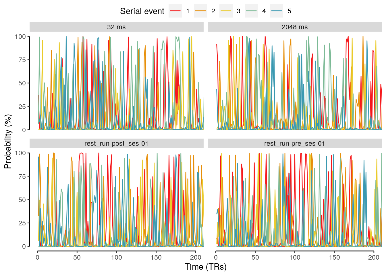
2.9.3 Calculating sequentiality
We create a function to determine whether a certain sequential combination of the task stimuli has been presented to the participants on sequence trials or not:
did_you_see_that <- function(seq, dt_events_seq) {
dt_events_seq_sub <- dt_events_seq %>%
#filter(subject == sub) %>%
setDT(.) %>%
# calculate if the input sequence was seen for every trial:
.[, by = .(subject, interval_time, trial), .(
num_events = .N,
seen = as.numeric(all(stim_label[serial_position] == seq))
)] %>%
# check if the number of events per sequence is 5:
verify(num_events == 5) %>%
# the number a seen sequences should be either 0 (not seen) or 5 (seen five)
# time for the five different speed conditions:
verify(.[, by = .(subject), .(sum_seen = sum(seen))]$sum_seen %in% c(0, 5)) %>%
# for each speed condition, the number should be 1 (seen) or 0 (not seen):
verify(.[, by = .(subject, interval_time), .(sum_seen = sum(seen))]$sum_seen %in% c(0, 1))
# return if sequence was seen (1) or not (0):
seen <- as.numeric(sum(dt_events_seq_sub$seen) == 5)
return(seen)
}We verify that the function works properly:
sequences = permn(1:5, sort = TRUE)
# list of all possible stimuli:
seq <- c("cat", "chair", "face", "house", "shoe")
# select one example participant:
sub = "sub-14"
# determine if participant saw 15 combinations of the five stimuli:
sum_seq = sum(unlist(lapply(X = sequences, function(x)
did_you_see_that(seq = seq[x], subset(dt_events_seq, subject == sub)))))
verify(data.table(sum_seq), sum_seq == 15)## sum_seq
## 1: 15We calculate the regression slopes for every TR and assumed sequence in resting-state data:
# create an array with all the stimulus labels:
stimuli <- c("cat", "chair", "face", "house", "shoe")
# register the computation start time:
start_time <- Sys.time()
# calculate sd probability, slope for every permutation of a sequence:
dt_pred_conc_slope_rest = dt_pred_conc %>%
# filter for resting state analyses only:
filter(stringr::str_detect(tITI, "rest")) %>%
setDT(.) %>%
# calculate sd probability, slope and if sequence was seen or not:
.[, by = .(id, classification, tITI, trial_tITI, seq_tr), .(
# calculate the number of events per TR and the mean position:
num_events = .N,
mean_position = mean(position),
# calculate the standard deviation of the probabilities:
sd_prob = sd(probability),
# calculate the slope for each permuted sequence:
slope = unlist(lapply(sequences, function(x) coef(lm(probability ~ x))[2] * (-1))),
# determine if the permuted sequence was actually seen by the subject:
seen = unlist(lapply(sequences, function(x)
did_you_see_that(seq = stimuli[x], subset(dt_events_seq, subject == unique(id)))))
)] %>%
# add a counter for all sequential combinations:
.[, by = .(id, classification, tITI, trial_tITI, seq_tr), "sequence" := seq(1,.N)]
# stop the counter and print the calculation time:
end_time = Sys.time()
print(end_time - start_time)We calculate the regression slopes for sequence data:
dt_pred_conc_slope_seq = dt_pred_conc %>%
# filter for sequence data only:
filter(!stringr::str_detect(tITI, "rest")) %>%
base::droplevels() %>%
setDT(.) %>%
# calculate the slope for every participant, speed and TR:
.[, by = .(id, classification, tITI, trial_tITI, seq_tr), .(
# calculate the number of events per TR and the mean position:
num_events = .N,
mean_position = mean(position),
# calculate the standard deviation of the probabilities:
sd_prob = sd(probability),
# calculate the slope for each permuted sequence:
slope = coef(lm(probability ~ position))[2] * (-1)
)] %>%
# add variables if sequence was seen or not and sequence counter:
.[, "seen" := 1] %>%
.[, "sequence" := 1]We combine the resting state and sequence trial slope data:
dt_pred_conc_slope = rbind(dt_pred_conc_slope_seq, dt_pred_conc_slope_rest) %>%
# verify that there are 5 events per TR and their mean position is 5:
verify(all(num_events == 5)) %>%
verify(all(mean_position == 3)) %>%
# sort the columns by classification approach, id, speed, trial and TR:
setorder(classification, id, tITI, trial_tITI, seq_tr) %>%
# add trial counter for every speed condition (and sequence):
.[stringr::str_detect(tITI, "rest"),
by = .(classification, id, tITI, sequence), ":=" (t = seq(1, .N))] %>%
.[!stringr::str_detect(tITI, "rest"),
by = .(classification, id, tITI), ":=" (t = seq(1, .N))] %>%
# group by classification, id, speed and trial and calculate step sizes:
.[!stringr::str_detect(tITI, "rest"), by = .(classification, id, tITI),
trial_start := trial_tITI - shift(trial_tITI)] %>%
# create a variable that signifies the trial starts for sequence trials:
transform(trial_start = ifelse(
is.na(trial_start) & !stringr::str_detect(tITI, "rest"), 1, trial_start)) %>%
# create new variable names for resting state data:
.[tITI == "rest_run-pre_ses-01", tITI := "Rest Pre S1"] %>%
.[tITI == "rest_run-post_ses-01", tITI := "Rest Post S1"] %>%
.[tITI == "rest_run-pre_ses-02", tITI := "Rest Pre S2"] %>%
.[tITI == "rest_run-post_ses-02", tITI := "Rest Post S2"] %>%
# sort the factor levels of the speed conditions:
transform(tITI = factor(tITI, levels = c(
"32 ms", "2048 ms", "Rest Pre S1", "Rest Post S1",
"Rest Pre S2", "Rest Post S2"))) %>%
# rename the factor for seen (1) and unseen (0) sequences:
.[, seen := ifelse(seen == 1, "More frequent", "Less frequent")] %>%
setDT(.)We save the regression slope data during manual execution, save it to the repository and reload it for all following analyses:
save(dt_pred_conc_slope, file = file.path(path_root, "data", "tmp", "dt_pred_conc_slope.Rdata"))load(file.path(path_root, "data", "tmp", "dt_pred_conc_slope.Rdata"))2.9.4 Mean slope coefficients
2.9.4.1 Fixed event order
We calculate the mean slope coefficients assuming a fixed ordering of sequence events for sequence trials:
# calculate the mean slope across participants for each time point:
dt_pred_conc_slope_mean <- dt_pred_conc_slope %>%
filter(sequence == 1) %>%
setDT(.) %>%
.[, by = .(classification, tITI, t, trial_start), .(
num_subs = .N,
mean_slope = mean(slope),
sem_upper = mean(slope) + (sd(slope)/sqrt(.N)),
sem_lower = mean(slope) - (sd(slope)/sqrt(.N))
)] %>%
verify(all(num_subs == 32)) %>%
filter(classification == "ovr") %>%
# sort the factor levels of the speed conditions:
transform(tITI = factor(tITI, levels = c(
"2048 ms", "32 ms", "Rest Pre S1", "Rest Post S1",
"Rest Pre S2", "Rest Post S2"))) %>%
setDT(.)2.9.4.2 Figure 5c
We plot the mean regression coefficient separately for all sequence speed conditions and the pre-task resting state data. Trial boundaries (for sequence trials) are shown as gray vertical lines.
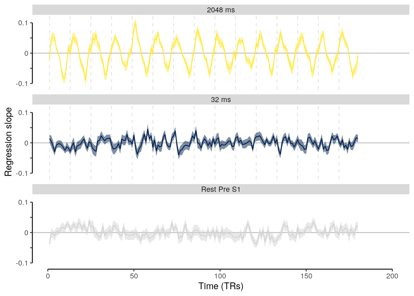
2.9.4.3 Source Data File Fig. 5c
dt_pred_conc_slope_mean %>% filter(tITI != "Rest Post S1") %>%
select(-num_subs, -classification) %>%
write.csv(., file = file.path(path_sourcedata, "source_data_figure_5c.csv"),
row.names = FALSE)We calculate the mean regression slopes and compare sequence and rest:
# calculate mean regression slopes for fast and slow sequence trials and rest:
dt_pred_conc_slope_stat = dt_pred_conc_slope %>%
filter(sequence == 1) %>%
setDT(.) %>%
.[, by = .(classification, id, tITI), .(
num_trs = .N,
mean_abs_slope = mean(abs(slope)),
abs_mean_slope = abs(mean(slope)),
mean_sd_prob = mean(sd_prob)
)] %>% verify(all(num_trs == 180)) %>%
filter(classification == "ovr") %>%
transform(tITI = factor(tITI, levels = c(
"32 ms", "2048 ms", "Rest Pre S1", "Rest Post S1",
"Rest Pre S2", "Rest Post S2"))) %>%
setDT(.)# compare mean probabilities between resting state and fast sequence data:
mean_sd_rest_pre = subset(dt_pred_conc_slope_stat, tITI == "Rest Pre S1")$mean_sd_prob
mean_sd_rest_post = subset(dt_pred_conc_slope_stat, tITI == "Rest Post S1")$mean_sd_prob
mean_sd_fast = subset(dt_pred_conc_slope_stat, tITI == "32 ms")$mean_sd_prob
mean_sd_slow = subset(dt_pred_conc_slope_stat, tITI == "2048 ms")$mean_sd_prob
fast_vs_rest_pre = t.test(x = mean_sd_rest_pre, y = mean_sd_fast, alternative = "two.sided", paired = TRUE)
fast_vs_rest_post = t.test(x = mean_sd_rest_post, y = mean_sd_fast, alternative = "two.sided", paired = TRUE)
fast_vs_slow = t.test(x = mean_sd_slow, y = mean_sd_fast, alternative = "two.sided", paired = TRUE)
slow_vs_rest_pre = t.test(x = mean_sd_rest_pre, y = mean_sd_slow, alternative = "two.sided", paired = TRUE)
rest_pre_vs_rest_post = t.test(x = mean_sd_rest_pre, y = mean_sd_rest_post, alternative = "two.sided", paired = TRUE)
print(round(c(mean(mean_sd_rest_pre), mean(mean_sd_fast), mean(mean_sd_slow)), 2))
round_pvalues(p.adjust(
c(fast_vs_rest_pre$p.value, fast_vs_slow$p.value, slow_vs_rest_pre$p.value,
rest_pre_vs_rest_post$p.value, fast_vs_rest_post$p.value), method = "fdr"))
cohensd_rest = round((mean(mean_sd_rest_pre) - mean(mean_sd_fast)) / sd(mean_sd_rest_pre - mean_sd_fast), 2)
cohensd_slow = round((mean(mean_sd_slow) - mean(mean_sd_fast)) / sd(mean_sd_slow - mean_sd_fast), 2)
print(cohensd_rest); print(cohensd_slow)
fast_vs_rest_pre; fast_vs_slow## [1] 0.23 0.20 0.22
## [1] "p < .001" "p < .001" "p = .19" "p = .18" "p = .002"
## [1] 0.88
## [1] 0.74
##
## Paired t-test
##
## data: mean_sd_rest_pre and mean_sd_fast
## t = 4.9859, df = 31, p-value = 2.236e-05
## alternative hypothesis: true difference in means is not equal to 0
## 95 percent confidence interval:
## 0.01724796 0.04112626
## sample estimates:
## mean of the differences
## 0.02918711
##
##
## Paired t-test
##
## data: mean_sd_slow and mean_sd_fast
## t = 4.1704, df = 31, p-value = 0.000227
## alternative hypothesis: true difference in means is not equal to 0
## 95 percent confidence interval:
## 0.009556449 0.027850046
## sample estimates:
## mean of the differences
## 0.018703252.9.4.4 Figure 5a / 5b
We plot the mean absolute regression slope for all speed conditions and pre-task resting state data:
plot_means = function(data, variable, ylabel, ylim){
#colors = c(hcl.colors(5, "Cividis")[c(1)], "gold", "gray")
colors = c(hcl.colors(5, "Cividis")[c(1)], "gold", grays(4))
fig_mean_beta = ggplot(
data = data %>% filter(tITI != "Rest Post S1"),
aes(
y = get(variable), x = tITI, fill = tITI)) +
geom_bar(stat = "summary", fun = "mean", position = position_dodge(0.9)) +
geom_point(position = position_jitter(width = 0.1, height = 0, seed = 2),
alpha = 1, inherit.aes = TRUE, pch = 21,
color = "white") +
stat_summary(fun.data = mean_se, geom = "errorbar",
position = position_dodge(0.9), width = 0, color = "black") +
xlab("Data") + ylab(ylabel) +
coord_capped_cart(left = "both", expand = TRUE, ylim = ylim) +
scale_fill_manual(values = colors, guide = FALSE) +
theme(axis.ticks.x = element_blank(), axis.line.x = element_blank(),
axis.title.x = element_blank()) +
theme(axis.text.x = element_text(angle = 45, hjust = 0.9)) +
theme(panel.border = element_blank(), axis.line.y = element_line()) +
theme(axis.line.y = element_line(colour = "black"),
panel.grid.major = element_blank(),
panel.grid.minor = element_blank(),
panel.background = element_blank())
}
fig_mean_beta = plot_means(data = dt_pred_conc_slope_stat, variable = "abs_mean_slope",
ylabel = "Absolute mean regression slope", ylim = c(0, 0.02))
fig_mean_beta_abs = plot_means(data = dt_pred_conc_slope_stat, variable = "mean_abs_slope",
ylabel = "Regression slope (abs)", ylim = c(0, 0.1))
fig_sd_prob = plot_means(data = dt_pred_conc_slope_stat, variable = "mean_sd_prob",
ylabel = "SD of probability", ylim = c(0, 0.4))
fig_mean_beta; fig_mean_beta_abs; fig_sd_prob;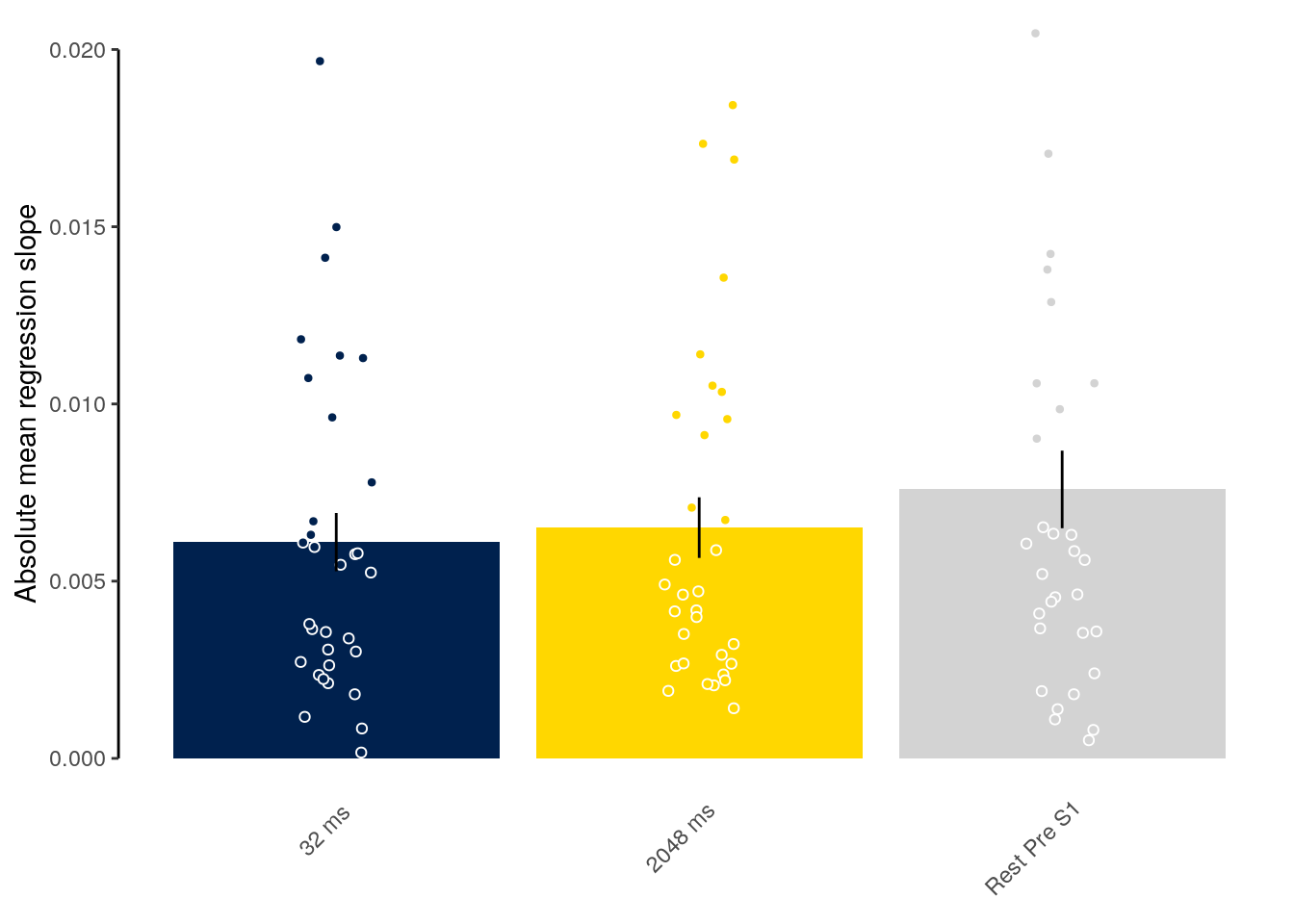
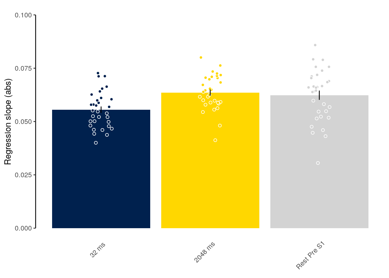
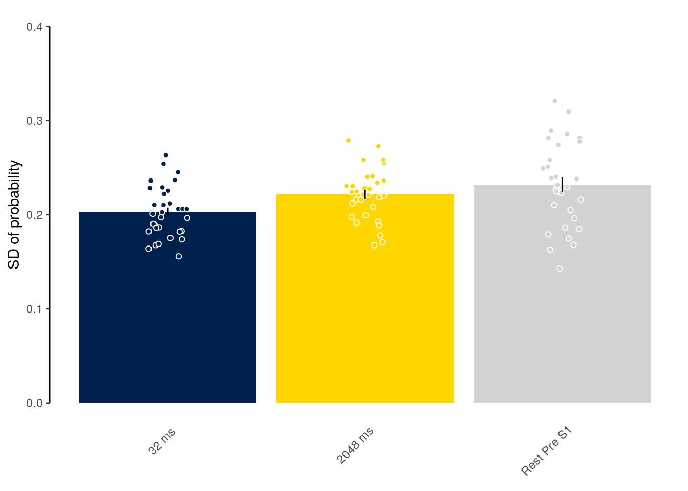
2.9.4.5 Source Data File Fig. 5a / 5b
dt_pred_conc_slope_stat %>%
select(-classification, -num_trs) %>%
write.csv(., file = file.path(path_sourcedata, "source_data_figure_5a.csv"),
row.names = FALSE)
dt_pred_conc_slope_stat %>%
select(-classification, -num_trs) %>%
write.csv(., file = file.path(path_sourcedata, "source_data_figure_5b.csv"),
row.names = FALSE)2.9.4.6 All possible event orders
We calculate the mean slope for every time point (for every TR) depending on if a sequence was actually seen or not (relevant for resting state data). Note, that by this definition, all sequences on sequence trials were “seen”.
# calculate the mean slope across participants for each time point:
dt_pred_conc_slope_mean_seen <- dt_pred_conc_slope %>%
# average slopes for each participant and each time point:
.[, by = .(id, classification, tITI, t, trial_start, seen), .(
num_seq = .N,
mean_slope_sub = mean(slope)
)] %>%
# number of sequences will be 1 (sequence conditions), 15 (seen permuted
# sequence condition), or 105 (not seen permuted sequence conditions):
verify(num_seq %in% c(1, 15, 105)) %>%
# calculate the mean slope across participants (including SEM):
.[, by = .(classification, tITI, t, trial_start, seen), .(
num_subs = .N,
mean_slope = mean(mean_slope_sub),
sem_upper = mean(mean_slope_sub) + (sd(mean_slope_sub)/sqrt(.N)),
sem_lower = mean(mean_slope_sub) - (sd(mean_slope_sub)/sqrt(.N))
)] %>%
# verify that data was averaged across the correct number of participants:
verify(all(num_subs == 32)) %>%
filter(classification == "ovr") %>%
# sort factor levels of the speed condition:
transform(tITI = factor(tITI, levels = c(
"2048 ms", "32 ms", "Rest Pre S1", "Rest Post S1",
"Rest Pre S2", "Rest Post S2"))) %>%
setDT(.)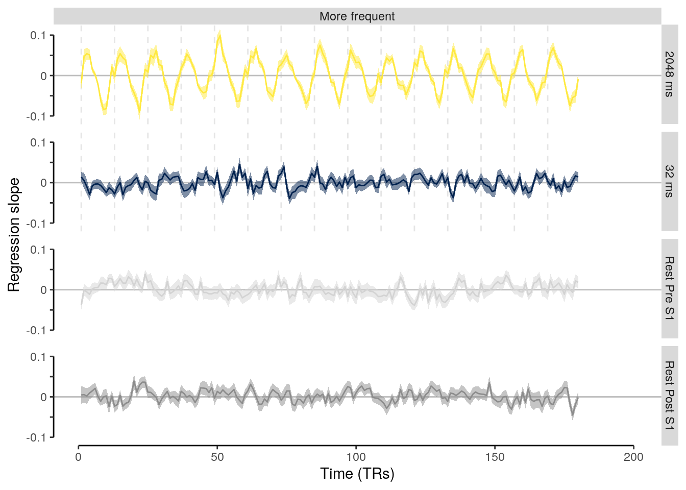
We calculate the mean absolute and non-absolute slopes for sequence and rest trials depending on whether the permuted sequence was actually seen or not:
# calculate mean regression slopes for fast and slow sequence trials and rest:
dt_pred_conc_slope_stat_seen = dt_pred_conc_slope %>%
.[, by = .(classification, id, tITI, seen), .(
num_trs = .N,
mean_slope = mean(slope),
mean_abs_slope = mean(abs(slope)),
abs_mean_slope = abs(mean(slope)),
abs_pos_slope = mean(abs(slope[slope > 0])),
abs_neg_slope = mean(abs(slope[slope < 0])),
mean_sd_prob = mean(sd_prob)
)] %>%
# check if the average slope was calculated across the correct number of TRs
# which should be 180 for sequence trials and 180 times number of sequences
# not seen (105) and 180 times sequences seen (15) in permuted rest data:
verify(all(num_trs %in% c(180, 180 * (120 - 15), 180 * 15))) %>%
filter(classification == "ovr") %>%
setDT(.)plot_means_seen = function(data, variable, ylabel, ylim){
#colors = c(hcl.colors(5, "Cividis")[c(1)], "gold", "gray")
grays = colorRampPalette(c("lightgray", "black"))
colors = c(hcl.colors(5, "Cividis")[c(1)], "gold", grays(4))
fig_mean_beta = ggplot(data = data, aes(
y = get(variable), x = tITI, fill = tITI)) +
facet_wrap(~ seen) +
geom_bar(stat = "summary", fun = "mean", position = position_dodge(0.9)) +
geom_point(position = position_jitter(width = 0.1, height = 0, seed = 2),
alpha = 1, inherit.aes = TRUE, pch = 21,
color = "white") +
stat_summary(fun.data = mean_se, geom = "errorbar",
position = position_dodge(0.9), width = 0, color = "black") +
xlab("Data") + ylab(ylabel) +
coord_capped_cart(left = "both", expand = TRUE, ylim = ylim) +
scale_fill_manual(values = colors, guide = FALSE) +
theme(axis.ticks.x = element_blank(), axis.line.x = element_blank(),
axis.title.x = element_blank()) +
theme(axis.text.x = element_text(angle = 45, hjust = 0.9)) +
theme(panel.border = element_blank(), axis.line.y = element_line()) +
theme(axis.line.y = element_line(colour = "black"),
panel.grid.major = element_blank(),
panel.grid.minor = element_blank(),
panel.background = element_blank())
}
fig_mean_beta_seen = plot_means_seen(
data = dt_pred_conc_slope_stat_seen, variable = "abs_mean_slope",
ylabel = "Absolute mean regression slope", ylim = c(-0.01, 0.02))
fig_mean_beta_abs_seen = plot_means_seen(
data = dt_pred_conc_slope_stat_seen, variable = "mean_abs_slope",
ylabel = "Mean absolute regression slope", ylim = c(0, 0.1))
fig_sd_prob_seen = plot_means_seen(
data = dt_pred_conc_slope_stat_seen, variable = "mean_sd_prob",
ylabel = "SD of probability", ylim = c(0, 0.4))
fig_mean_pos_abs_seen = plot_means_seen(
data = dt_pred_conc_slope_stat_seen, variable = "abs_pos_slope",
ylabel = "Mean absolute regression slope", ylim = c(0, 0.1))
fig_mean_neg_abs_seen = plot_means_seen(
data = dt_pred_conc_slope_stat_seen, variable = "abs_neg_slope",
ylabel = "Mean absolute regression slope", ylim = c(0, 0.1))
fig_mean_slope_seen = plot_means_seen(
data = dt_pred_conc_slope_stat_seen, variable = "mean_slope",
ylabel = "Absolute mean regression slope", ylim = c(-0.01, 0.02))
fig_mean_beta_seen; fig_mean_beta_abs_seen; fig_sd_prob_seen;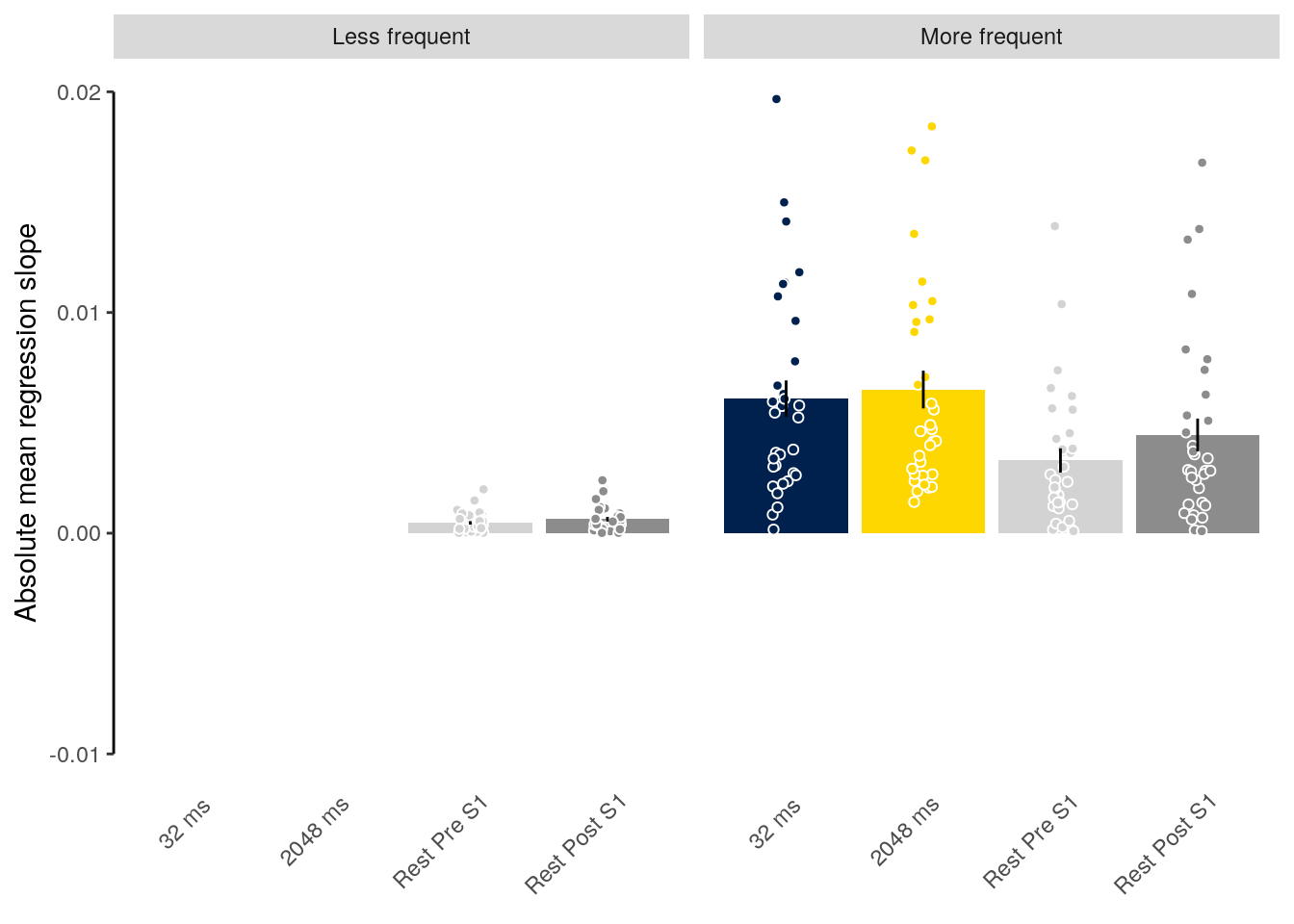

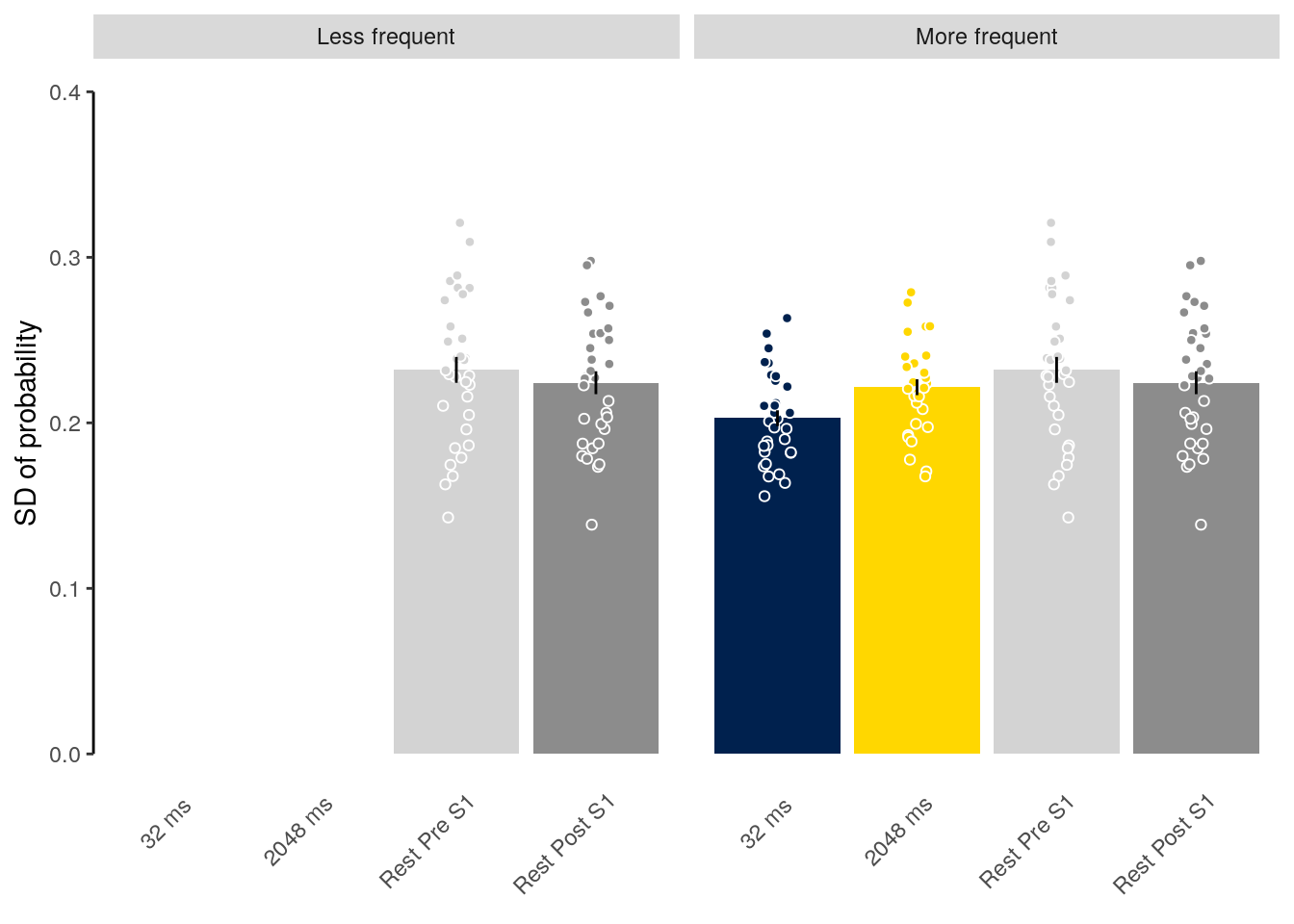
fig_mean_pos_abs_seen; fig_mean_neg_abs_seen; fig_mean_slope_seen
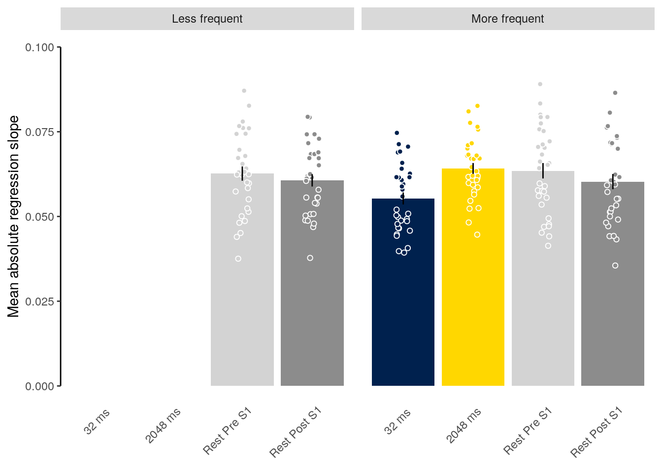
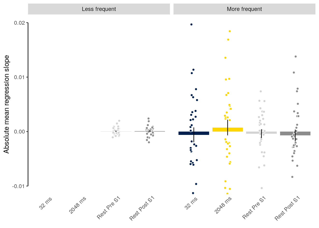
2.9.5 Frequency spectrum analyses
2.9.5.1 Fixed event order
We create a data table with frequency expectations:
fitfreq = 1 / 5.26
stim_dur = 0.1
num_seq_stim = 5
# calculate the delta
delta_freq_fast = fitfreq / (1 + fitfreq * (
num_seq_stim * stim_dur + (num_seq_stim - 1) * 0.032))
delta_freq_slow = fitfreq / (1 + fitfreq * (
num_seq_stim * stim_dur + (num_seq_stim - 1) * 2.048))
delta_freq_rest = 0.01
# create a data table with the expected frequencies:
frequency_expectation = data.table(xintercept = c(
delta_freq_fast, delta_freq_slow, rep(delta_freq_rest, 4)))We calculate the frequency spectra based on the time courses of regression slope coefficients:
library(lomb)
# create a time vector with random gaps:
time_concat = as.vector(sapply(0:14, FUN = function(x) seq(0, 1*11, by = 1) + x*100 + round(runif(1)*50)))
# get the frequency spectrum of fast and slow trials:
dt_pred_rest_lsp = dt_pred_conc_slope %>%
filter(sequence == 1) %>%
setDT(.) %>%
.[, by = .(classification, id, tITI), {
frequency_spectrum = lsp(x = slope, times = time_concat, from = 0, to = 0.3, plot = FALSE)
list(num_trs = .N, freq_bins = frequency_spectrum$scanned,
filter_width = round(0.01/mean(diff(frequency_spectrum$scanned))),
power = frequency_spectrum$power
)}] %>% verify(all(num_trs == 180)) %>% verify(length(unique(filter_width)) == 1) %>%
# smooth the frequency spectra and frequency bins:
.[, by = .(classification, id, tITI), ":=" (
power_smooth = stats::filter(power, rep(1/unique(filter_width), unique(filter_width))),
freq_bins_smooth = stats::filter(freq_bins, rep(1/unique(filter_width), unique(filter_width)))
)]# calculate the mean frequency profile across participants:
dt_pred_rest_lsp_mean = dt_pred_rest_lsp %>%
# filter out NA frequency spectrum:
filter(!is.na(power_smooth)) %>%
setDT(.) %>%
# calculate the mean smoothed frequency spectrum across all frequency bins:
.[, by = .(classification, tITI, freq_bins_smooth), .(
num_subs = .N,
mean_spec = mean(power_smooth),
sem_upper = mean(power_smooth) + (sd(power_smooth)/sqrt(.N)),
sem_lower = mean(power_smooth) - (sd(power_smooth)/sqrt(.N))
)] %>%
verify(all(num_subs == 32))2.9.5.2 Figure 5d
#colors = c(hcl.colors(5, "Cividis")[c(1)], "gold", "gray")
colors = c(hcl.colors(5, "Cividis")[c(1)], "gold", grays(1), "black", grays(2))
fig_freq_lsp = ggplot(
data = dt_pred_rest_lsp_mean %>% filter(tITI != "Rest Post S1"),
aes(
color = tITI, y = as.numeric(mean_spec), x = as.numeric(freq_bins_smooth))) +
geom_vline(data = frequency_expectation, aes(xintercept = xintercept),
linetype = "dashed", color = colors) +
geom_line() +
geom_ribbon(aes(fill = tITI, ymin = sem_lower, ymax = sem_upper),
alpha = 0.3, color = NA) +
geom_text(data = frequency_expectation, aes(
x = xintercept + 0.02, y = 0.1, label = paste(round(xintercept, 2))),
color = colors) +
xlab("Frequency") + ylab("Power") +
scale_color_manual(name = "", values = colors) +
scale_fill_manual(name = "", values = colors) +
theme(legend.position = "top", legend.direction = "horizontal",
legend.justification = "center", legend.margin = margin(0, 0, 0, 0),
legend.box.margin = margin(t = 0, r = 0, b = -5, l = 0)) +
coord_capped_cart(left = "both", bottom = "both", expand = TRUE,
ylim = c(0, 3), xlim = c(0, 0.3)) +
guides(color = guide_legend(nrow = 1)) +
scale_x_continuous(labels = label_fill(seq(0, 0.3, by = 0.05), mod = 1),
breaks = seq(0, 0.3, by = 0.05)) +
theme(panel.border = element_blank(), axis.line = element_line()) +
theme(axis.line = element_line(colour = "black"),
panel.grid.major = element_blank(),
panel.grid.minor = element_blank(),
panel.border = element_blank(),
panel.background = element_blank())
fig_freq_lsp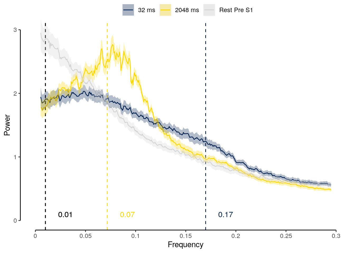
2.9.5.3 Source Data File Fig. 5d
dt_pred_rest_lsp_mean %>% filter(tITI != "Rest Post S1") %>%
select(- classification, -num_subs) %>%
write.csv(., file = file.path(path_sourcedata, "source_data_figure_5d.csv"),
row.names = FALSE)2.9.5.4 All possible event orders
We calculate the frequency spectrum for all permuted resting state sequences and sequence trials:
# create a time vector with random gaps:
time_concat = as.vector(sapply(0:14, FUN = function(x) seq(0, 1*11, by = 1) + x*100 + round(runif(1)*50)))
# get the frequency spectrum of fast and slow trials:
dt_pred_rest_lsp_seen = dt_pred_conc_slope %>%
# calculate the frequency spectrum for each permuted sequence and participant:
.[, by = .(classification, id, tITI, sequence, seen), {
frequency_spectrum = lomb::lsp(
x = slope, times = time_concat, from = 0, to = 0.3, plot = FALSE)
list(num_trs = .N, freq_bins = frequency_spectrum$scanned,
filter_width = round(0.01/mean(diff(frequency_spectrum$scanned))),
power = frequency_spectrum$power
)}] %>%
# the number of TRs for each stretch of activation patterns should be 180:
verify(all(num_trs == 180)) %>%
# there should only be one filtering width per sequence:
verify(length(unique(filter_width)) == 1) %>%
# there should be 120 sequence permutations in the resting condition:
verify(.[, by = .(classification, id, tITI), .(
num_seq = length(unique(sequence)))]$num_seq %in% c(1, 120)) %>%
# smooth the frequency spectra and frequency bins:
.[, by = .(classification, id, tITI, sequence, seen), ":=" (
power_smooth = stats::filter(power, rep(1/unique(filter_width), unique(filter_width))),
freq_bins_smooth = stats::filter(freq_bins, rep(1/unique(filter_width), unique(filter_width)))
)]We calculate the mean frequency spectra for each participant, classification approach, speed condition, smoothed frequency bin and if the (permuted) rest sequence was actually seen during the task or not:
# calculate the mean frequency profile across participants:
dt_pred_rest_lsp_mean_seen = dt_pred_rest_lsp_seen %>%
# filter out NA frequency spectrum:
filter(!is.na(power_smooth)) %>%
setDT(.) %>%
# calculate the mean smoothed frequency spectrum across all frequency bins and sequences:
.[, by = .(classification, id, tITI, freq_bins_smooth), .(
num_seqs = .N,
power_smooth = mean(power_smooth)
)] %>%
# the number of sequences should be 1 for sequence trials, 15 for seen
# permuted rest repetitions and 105 for unseen sequence repetitions:
verify(num_seqs %in% c(1, 120)) %>%
# calculate the mean smoothed frequency spectrum across all frequency bins:
.[, by = .(classification, tITI, freq_bins_smooth), .(
num_subs = .N,
mean_spec = mean(power_smooth),
sem_upper = mean(power_smooth) + (sd(power_smooth)/sqrt(.N)),
sem_lower = mean(power_smooth) - (sd(power_smooth)/sqrt(.N))
)] %>%
# verify if data was averaged across the expected number of participants:
verify(all(num_subs == 32))calc_delta <- function(speed_s) {
# input speed_s: sequence speed (ISI), in seconds
fitfreq = 1 / 5.26
stim_dur = 0.1
num_seq_stim = 5
delta = fitfreq / (1 + fitfreq * (num_seq_stim * stim_dur + (num_seq_stim - 1) * speed_s))
return(delta)
}
# create a data table with the expected frequencies:
frequency_expectation = data.table(xintercept = c(
calc_delta(0.032), calc_delta(2.048), 0.01),
tITI = c("32 ms", "2048 ms", "Rest Pre S1"))2.9.5.5 Figure 6a
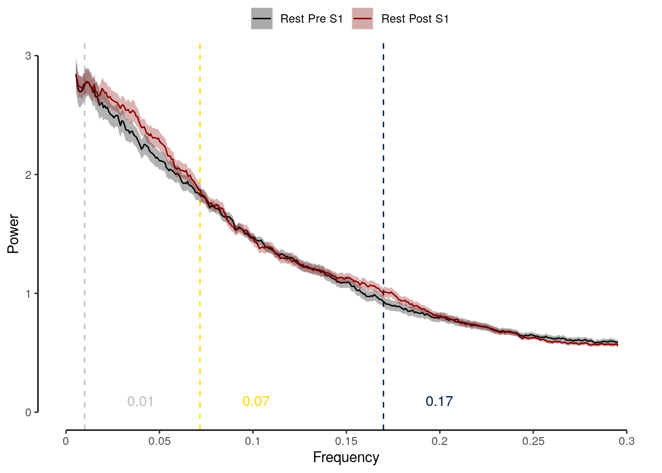
2.9.5.6 Source Data File Fig. 6a
dt_pred_rest_lsp_mean_seen %>%
filter(tITI %in% c("Rest Pre S1", "Rest Post S1")) %>%
select(-classification, -num_subs) %>%
write.csv(., file = file.path(path_sourcedata, "source_data_figure_6a.csv"),
row.names = FALSE)We calculate the relative power (difference between pre- and post task resting state data) across the entire frequency spectrum:
# calculate the mean frequency profile across participants:
dt_pred_rest_lsp_mean_rel_seen = dt_pred_rest_lsp_seen %>%
filter(tITI %in% c("Rest Pre S1", "Rest Post S1")) %>%
transform(tITI = ifelse(tITI == "Rest Pre S1", "rest_pre_s1", "rest_post_s1")) %>%
# filter out NA frequency spectrum:
filter(!is.na(power_smooth)) %>%
setDT(.) %>%
# calculate the mean smoothed frequency spectrum across all frequency bins and sequences:
.[, by = .(classification, id, tITI, freq_bins_smooth), .(
num_seqs = .N,
power_smooth = mean(power_smooth)
)] %>%
# the number of sequences should be 1 for sequence trials, 15 for seen
# permuted rest repetitions and 105 for unseen sequence repetitions:
verify(num_seqs %in% c(1, 120)) %>%
# transform resting state data from long to wide to calculate relative power:
spread(data = ., key = tITI, value = power_smooth) %>%
mutate(rel_power = rest_post_s1 - rest_pre_s1) %>%
setDT(.) %>%
# calculate the mean smoothed frequency spectrum across all frequency bins:
.[, by = .(classification, freq_bins_smooth), .(
num_subs = .N,
mean_spec = mean(rel_power),
sem_upper = mean(rel_power) + (sd(rel_power)/sqrt(.N)),
sem_lower = mean(rel_power) - (sd(rel_power)/sqrt(.N))
)] %>%
# verify if data was averaged across the expected number of participants:
verify(all(num_subs == 32))We determine in which frequency range the peak in difference between pre- and post-task rest is:
increase_slow = round(dt_pred_rest_lsp_mean_rel_seen$freq_bins_smooth[which.max(dt_pred_rest_lsp_mean_rel_seen$mean_spec)], 2)
increase_fast = round(dt_pred_rest_lsp_mean_rel_seen$freq_bins_smooth[dt_pred_rest_lsp_mean_rel_seen$freq_bins_smooth > 0.07][which.max(dt_pred_rest_lsp_mean_rel_seen[dt_pred_rest_lsp_mean_rel_seen$freq_bins_smooth > 0.07]$mean_spec)], 2)
increase_slow; increase_fast;## [1] 0.04## [1] 0.172.9.5.7 Figure 6b
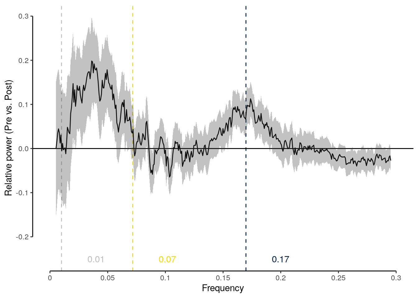
2.9.5.8 Source Data File Fig. 6b
dt_pred_rest_lsp_mean_rel_seen %>%
select(-classification, -num_subs) %>%
write.csv(., file = file.path(path_sourcedata, "source_data_figure_6b.csv"),
row.names = FALSE)2.9.5.9 Frequency spectra of frequent vs. less frequent sequences
We calculate the mean frequency spectra depending on whether the assumed sequences occured more frequency or less frequently during the task:
# calculate the mean frequency profile across participants:
dt_pred_rest_lsp_mean_seen = dt_pred_rest_lsp_seen %>%
# filter out NA frequency spectrum:
filter(!is.na(power_smooth)) %>%
setDT(.) %>%
# calculate the mean smoothed frequency spectrum across all frequency bins and sequences:
.[, by = .(classification, id, tITI, freq_bins_smooth, seen), .(
num_seqs = .N,
power_smooth = mean(power_smooth)
)] %>%
# the number of sequences should be 1 for sequence trials, 15 for seen
# permuted rest repetitions and 105 for unseen sequence repetitions:
verify(num_seqs %in% c(1, 15, 105)) %>%
# calculate the mean smoothed frequency spectrum across all frequency bins:
.[, by = .(classification, tITI, freq_bins_smooth, seen), .(
num_subs = .N,
mean_spec = mean(power_smooth),
sem_upper = mean(power_smooth) + (sd(power_smooth)/sqrt(.N)),
sem_lower = mean(power_smooth) - (sd(power_smooth)/sqrt(.N))
)] %>%
# verify if data was averaged across the expected number of participants:
verify(all(num_subs == 32))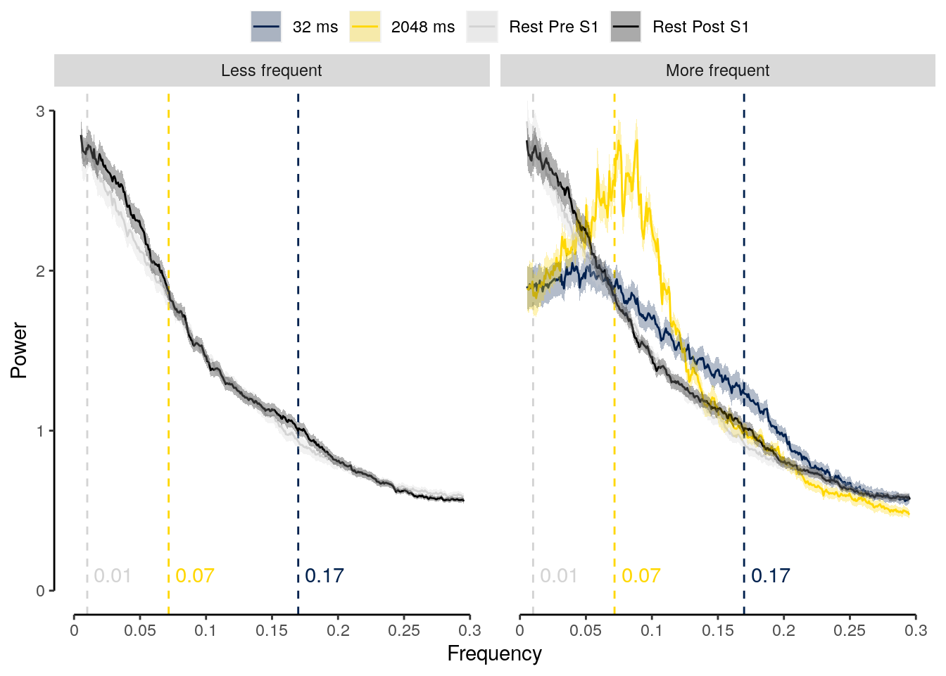
2.9.6 Relative frequency spectra (fixed order)
We compare the power of the expected frequencies of resting state, fast, and slow sequence trial data in data from resting state, fast, and slow sequence trial data.
fitfreq = 1 / 5.26
stim_dur = 0.1
num_seq_stim = 5
# calculate the delta
delta_freq_fast = fitfreq / (1 + fitfreq * (num_seq_stim * stim_dur + (num_seq_stim - 1) * 0.032))
delta_freq_slow = fitfreq / (1 + fitfreq * (num_seq_stim * stim_dur + (num_seq_stim - 1) * 2.048))
delta_freq_rest = 0.01
# create a data table with the expected frequencies:
frequency_expectation = data.table(xintercept = c(
delta_freq_fast, delta_freq_slow, rep(delta_freq_rest, 4)))dt_pred_rest_lsp_exp = dt_pred_rest_lsp %>%
.[, by = .(classification, id, tITI), .(
power_index_fast = power_smooth[which.min(abs(freq_bins_smooth - delta_freq_fast))],
power_index_slow = power_smooth[which.min(abs(freq_bins_smooth - delta_freq_slow))],
power_index_rest = power_smooth[which.min(abs(freq_bins_smooth - delta_freq_rest))]
)] %>%
# melt all index variables into one column:
gather(grep("power", names(.), fixed = TRUE), key = "index", value = "power") %>% setDT(.) %>%
.[grepl("index_fast", index), label := paste0("Fast (", round(delta_freq_fast, 2), ")")] %>%
.[grepl("index_slow", index), label := paste0("Slow (", round(delta_freq_slow, 2), ")")] %>%
.[grepl("index_rest", index), label := paste0("Rest (", round(delta_freq_rest, 2), ")")] %>%
setorder(., classification, id, tITI) %>%
filter(classification == "ovr") %>%
setDT(.)2.9.6.1 Figure 5e
colors = c(hcl.colors(5, "Cividis")[c(1)], "gold", "gray", "black")
fig_freq_exp = ggplot(
data = dt_pred_rest_lsp_exp %>% filter(tITI != "Rest Post S1"),
aes(y = power, x = fct_rev(label), fill = tITI)) +
geom_bar(stat = "summary", fun = "mean", position = position_dodge(0.9),
width = 0.8) +
geom_point(position = position_jitterdodge(
jitter.width = 0.1, jitter.height = 0, seed = 2, dodge.width = 0.9),
alpha = 1, inherit.aes = TRUE, pch = 21,
color = "white") +
stat_summary(fun.data = "mean_se", geom = "errorbar",
position = position_dodge(0.9), width = 0, color = "black") +
xlab("Predicted frequency") + ylab("Power") +
coord_capped_cart(left = "both", bottom = "both", expand = TRUE, ylim = c(0, 5)) +
scale_fill_manual(values = colors, name = "") +
theme(axis.ticks.x = element_line(color = "white"), axis.line.x = element_line(color = "white")) +
theme(legend.position = "top", legend.direction = "horizontal",
legend.justification = "center", legend.margin = margin(t = 0, r = 0, b = 0, l = 0),
legend.box.margin = margin(t = 0, r = 0, b = 0, l = 0)) +
theme(panel.border = element_blank(), axis.line = element_line()) +
theme(axis.line = element_line(colour = "black"),
panel.grid.major = element_blank(),
panel.grid.minor = element_blank(),
panel.border = element_blank(),
panel.background = element_blank())
fig_freq_exp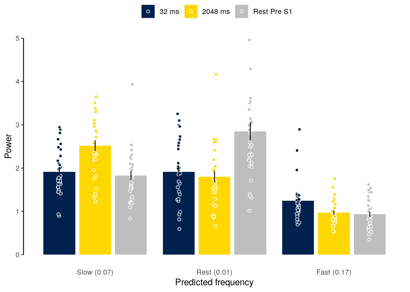
lme_power <- lmerTest::lmer(
power ~ tITI + (1 | id),
data = dt_pred_rest_lsp_exp %>%
filter(tITI != "Rest Post S1" & index == "power_index_fast"),
control = lcctrl)
summary(lme_power)
anova(lme_power)
emmeans_results = emmeans(lme_power, list(pairwise ~ tITI))
emmeans_results## Linear mixed model fit by REML. t-tests use Satterthwaite's method [
## lmerModLmerTest]
## Formula: power ~ tITI + (1 | id)
## Data: dt_pred_rest_lsp_exp %>% filter(tITI != "Rest Post S1" & index ==
## "power_index_fast")
## Control: lcctrl
##
## REML criterion at convergence: 86.8
##
## Scaled residuals:
## Min 1Q Median 3Q Max
## -1.5706 -0.6071 -0.1167 0.3281 4.1123
##
## Random effects:
## Groups Name Variance Std.Dev.
## id (Intercept) 0.02222 0.1491
## Residual 0.11422 0.3380
## Number of obs: 96, groups: id, 32
##
## Fixed effects:
## Estimate Std. Error df t value Pr(>|t|)
## (Intercept) 1.24805 0.06530 88.31374 19.113 < 2e-16 ***
## tITI2048 ms -0.27643 0.08449 62.00000 -3.272 0.001749 **
## tITIRest Pre S1 -0.31311 0.08449 62.00000 -3.706 0.000451 ***
## ---
## Signif. codes: 0 '***' 0.001 '**' 0.01 '*' 0.05 '.' 0.1 ' ' 1
##
## Correlation of Fixed Effects:
## (Intr) tITI2m
## tITI2048 ms -0.647
## tITIRstPrS1 -0.647 0.500
## Type III Analysis of Variance Table with Satterthwaite's method
## Sum Sq Mean Sq NumDF DenDF F value Pr(>F)
## tITI 1.8752 0.93759 2 62 8.2088 0.0006876 ***
## ---
## Signif. codes: 0 '***' 0.001 '**' 0.01 '*' 0.05 '.' 0.1 ' ' 1
## $`emmeans of tITI`
## tITI emmean SE df lower.CL upper.CL
## 32 ms 1.248 0.0653 88.3 1.118 1.38
## 2048 ms 0.972 0.0653 88.3 0.842 1.10
## Rest Pre S1 0.935 0.0653 88.3 0.805 1.06
##
## Degrees-of-freedom method: kenward-roger
## Confidence level used: 0.95
##
## $`pairwise differences of tITI`
## contrast estimate SE df t.ratio p.value
## 32 ms - 2048 ms 0.2764 0.0845 62 3.272 0.0049
## 32 ms - Rest Pre S1 0.3131 0.0845 62 3.706 0.0013
## 2048 ms - Rest Pre S1 0.0367 0.0845 62 0.434 0.9015
##
## Degrees-of-freedom method: kenward-roger
## P value adjustment: tukey method for comparing a family of 3 estimates# get the power spectrum of the expected fast frequency in fast data:
power_fast = subset(dt_pred_rest_lsp_exp, index == "power_index_fast" & tITI == "32 ms")$power
# get the power spectrum of the expected fast frequency in slow data:
power_slow = subset(dt_pred_rest_lsp_exp, index == "power_index_fast" & tITI == "2048 ms")$power
# get the power spectrum of the expected fast frequency in rest data:
power_rest_pre = subset(dt_pred_rest_lsp_exp, index == "power_index_fast" & tITI == "Rest Pre S1")$power
# compare fast vs. slow and fast vs. rest:
ttest_power_fastvsslow = t.test(power_fast, power_slow, paired = TRUE)
ttest_power_fastvsrestpre = t.test(power_fast, power_rest_pre, paired = TRUE)
ttest_power_slowvsrestpre = t.test(power_slow, power_rest_pre, paired = TRUE)
round_pvalues(p.adjust(c(ttest_power_fastvsslow$p.value,
ttest_power_fastvsrestpre$p.value,
ttest_power_slowvsrestpre$p.value), method = "fdr"))## [1] "p = .006" "p = .005" "p = .61"ttest_power_fastvsslow; ttest_power_fastvsrestpre; ttest_power_slowvsrestpre##
## Paired t-test
##
## data: power_fast and power_slow
## t = 3.109, df = 31, p-value = 0.004004
## alternative hypothesis: true difference in means is not equal to 0
## 95 percent confidence interval:
## 0.09509112 0.45776947
## sample estimates:
## mean of the differences
## 0.2764303##
## Paired t-test
##
## data: power_fast and power_rest_pre
## t = 3.4086, df = 31, p-value = 0.001829
## alternative hypothesis: true difference in means is not equal to 0
## 95 percent confidence interval:
## 0.1257631 0.5004613
## sample estimates:
## mean of the differences
## 0.3131122##
## Paired t-test
##
## data: power_slow and power_rest_pre
## t = 0.51505, df = 31, p-value = 0.6102
## alternative hypothesis: true difference in means is not equal to 0
## 95 percent confidence interval:
## -0.1085718 0.1819355
## sample estimates:
## mean of the differences
## 0.036681882.9.6.2 Source Data File Fig. 5e
dt_pred_rest_lsp_exp %>% filter(tITI != "Rest Post S1") %>%
select(-classification, -index) %>%
write.csv(., file = file.path(path_sourcedata, "source_data_figure_5e.csv"),
row.names = FALSE)2.9.7 Relative frequency spectra (all orders)
dt_pred_rest_lsp_exp_seen = dt_pred_rest_lsp_seen %>%
.[, by = .(classification, id, tITI, sequence, seen), .(
power_index_fast = power_smooth[which.min(abs(freq_bins_smooth - delta_freq_fast))],
power_index_slow = power_smooth[which.min(abs(freq_bins_smooth - delta_freq_slow))],
power_index_rest = power_smooth[which.min(abs(freq_bins_smooth - delta_freq_rest))]
)] %>%
# melt all index variables into one column:
gather(grep("power", names(.), fixed = TRUE), key = "index", value = "power") %>%
setDT(.) %>%
.[grepl("index_fast", index), label := paste0("Fast (", round(delta_freq_fast, 2), ")")] %>%
.[grepl("index_slow", index), label := paste0("Slow (", round(delta_freq_slow, 2), ")")] %>%
.[grepl("index_rest", index), label := paste0("Rest (", round(delta_freq_rest, 2), ")")] %>%
# average across sequences for seen and unseen sequences:
.[, by = .(classification, id, tITI, seen, index, label), .(
num_seqs = .N,
power = mean(power)
)] %>%
# check if the number of sequences matches for sequence (1), seen (15) and
# unseen (105) sequences in permuted resting state sequences:
verify(num_seqs %in% c(1, 15, 105)) %>%
setorder(., classification, id, tITI) %>%
filter(classification == "ovr") %>%
setDT(.)colors = c(hcl.colors(5, "Cividis")[c(1)], "gold", "gray", "black")
fig_freq_exp_seen = ggplot(data = dt_pred_rest_lsp_exp_seen, aes(
y = power, x = fct_rev(label), fill = tITI)) +
geom_bar(stat = "summary", fun = "mean", position = position_dodge(0.9),
width = 0.8) +
geom_point(position = position_jitterdodge(
jitter.width = 0.1, jitter.height = 0, seed = 2, dodge.width = 0.9),
alpha = 1, inherit.aes = TRUE, pch = 21,
color = "white") +
facet_wrap(~ seen) +
stat_summary(fun.data = "mean_se", geom = "errorbar",
position = position_dodge(0.9), width = 0, color = "black") +
xlab("Predicted frequency") + ylab("Power") +
coord_capped_cart(left = "both", bottom = "both", expand = TRUE, ylim = c(0, 5)) +
scale_fill_manual(values = colors, name = "") +
theme(axis.ticks.x = element_line(color = "white"), axis.line.x = element_line(color = "white")) +
theme(legend.position = "top", legend.direction = "horizontal",
legend.justification = "center", legend.margin = margin(t = 0, r = 0, b = 0, l = 0),
legend.box.margin = margin(t = 0, r = 0, b = 0, l = 0)) +
theme(panel.border = element_blank(), axis.line = element_line()) +
theme(axis.line = element_line(colour = "black"),
panel.grid.major = element_blank(),
panel.grid.minor = element_blank(),
panel.border = element_blank(),
panel.background = element_blank())
fig_freq_exp_seen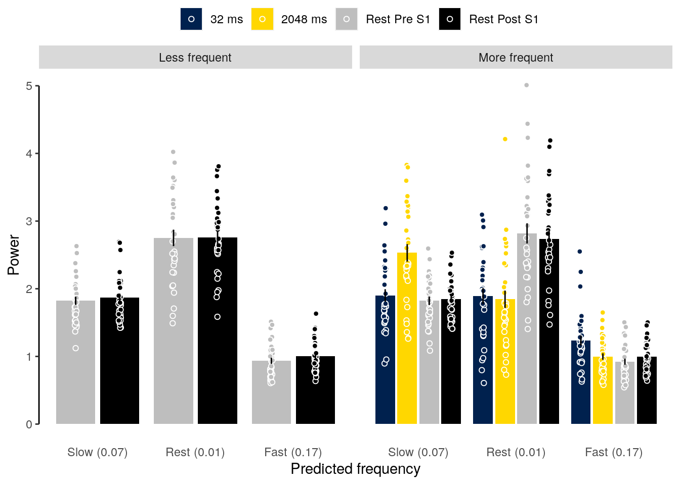
We examine the effect of resting-state session (pre- vs. post-task rest) and sequence frequency (less frequent vs. more frequent) on the power in the high frequency range (predicted by our model) indicative of fast sequential reactivation:
lme_power <- lmerTest::lmer(
power ~ tITI * seen + (tITI + seen | id),
data = subset(dt_pred_rest_lsp_exp_seen, index == "power_index_fast" &
stringr::str_detect(tITI, "Rest")),
control = lcctrl)
summary(lme_power)
anova(lme_power)
emmeans_results = emmeans(lme_power, list(pairwise ~ tITI | seen))
emmeans_results## Linear mixed model fit by REML. t-tests use Satterthwaite's method [
## lmerModLmerTest]
## Formula: power ~ tITI * seen + (tITI + seen | id)
## Data: subset(dt_pred_rest_lsp_exp_seen, index == "power_index_fast" &
## stringr::str_detect(tITI, "Rest"))
## Control: lcctrl
##
## REML criterion at convergence: -130
##
## Scaled residuals:
## Min 1Q Median 3Q Max
## -1.68077 -0.52070 0.01264 0.50310 1.59810
##
## Random effects:
## Groups Name Variance Std.Dev. Corr
## id (Intercept) 0.0653144 0.25557
## tITIRest Post S1 0.0575852 0.23997 -0.59
## seenMore frequent 0.0003235 0.01799 -1.00 0.51
## Residual 0.0033971 0.05828
## Number of obs: 128, groups: id, 32
##
## Fixed effects:
## Estimate Std. Error df t value
## (Intercept) 0.93509 0.04634 31.77642 20.180
## tITIRest Post S1 0.06523 0.04485 34.49637 1.454
## seenMore frequent -0.01262 0.01491 61.87659 -0.846
## tITIRest Post S1:seenMore frequent 0.01053 0.02061 62.00000 0.511
## Pr(>|t|)
## (Intercept) <2e-16 ***
## tITIRest Post S1 0.155
## seenMore frequent 0.401
## tITIRest Post S1:seenMore frequent 0.611
## ---
## Signif. codes: 0 '***' 0.001 '**' 0.01 '*' 0.05 '.' 0.1 ' ' 1
##
## Correlation of Fixed Effects:
## (Intr) tITIPS snMrfr
## tITIRstPsS1 -0.597
## seenMrfrqnt -0.361 0.262
## tITIRPS1:Mf 0.111 -0.230 -0.691
## Type III Analysis of Variance Table with Satterthwaite's method
## Sum Sq Mean Sq NumDF DenDF F value Pr(>F)
## tITI 0.0088584 0.0088584 1 31.000 2.6076 0.1165
## seen 0.0015829 0.0015829 1 52.988 0.4660 0.4978
## tITI:seen 0.0008864 0.0008864 1 62.000 0.2609 0.6113
## $`emmeans of tITI | seen`
## seen = Less frequent:
## tITI emmean SE df lower.CL upper.CL
## Rest Pre S1 0.935 0.0463 31.8 0.841 1.03
## Rest Post S1 1.000 0.0410 32.0 0.917 1.08
##
## seen = More frequent:
## tITI emmean SE df lower.CL upper.CL
## Rest Pre S1 0.922 0.0433 31.9 0.834 1.01
## Rest Post S1 0.998 0.0393 32.1 0.918 1.08
##
## Degrees-of-freedom method: kenward-roger
## Confidence level used: 0.95
##
## $`pairwise differences of tITI | seen`
## seen = Less frequent:
## contrast estimate SE df t.ratio p.value
## Rest Pre S1 - Rest Post S1 -0.0652 0.0449 34.4 -1.454 0.1549
##
## seen = More frequent:
## contrast estimate SE df t.ratio p.value
## Rest Pre S1 - Rest Post S1 -0.0758 0.0449 34.4 -1.689 0.1003
##
## Degrees-of-freedom method: kenward-rogerlme_power <- lmerTest::lmer(
power ~ tITI + (seen | id),
data = subset(dt_pred_rest_lsp_exp_seen, index == "power_index_fast" &
stringr::str_detect(tITI, "Rest")),
control = lcctrl)
summary(lme_power)
anova(lme_power)
emmeans_results = emmeans(lme_power, list(pairwise ~ tITI))
emmeans_results## Linear mixed model fit by REML. t-tests use Satterthwaite's method [
## lmerModLmerTest]
## Formula: power ~ tITI + (seen | id)
## Data: subset(dt_pred_rest_lsp_exp_seen, index == "power_index_fast" &
## stringr::str_detect(tITI, "Rest"))
## Control: lcctrl
##
## REML criterion at convergence: -52.1
##
## Scaled residuals:
## Min 1Q Median 3Q Max
## -1.9246 -0.6701 -0.1003 0.5636 2.1896
##
## Random effects:
## Groups Name Variance Std.Dev. Corr
## id (Intercept) 0.0382407 0.19555
## seenMore frequent 0.0002275 0.01508 -1.00
## Residual 0.0221629 0.14887
## Number of obs: 128, groups: id, 32
##
## Fixed effects:
## Estimate Std. Error df t value Pr(>|t|)
## (Intercept) 0.92784 0.03794 39.88504 24.453 < 2e-16 ***
## tITIRest Post S1 0.07049 0.02632 94.99805 2.679 0.00871 **
## ---
## Signif. codes: 0 '***' 0.001 '**' 0.01 '*' 0.05 '.' 0.1 ' ' 1
##
## Correlation of Fixed Effects:
## (Intr)
## tITIRstPsS1 -0.347
## Type III Analysis of Variance Table with Satterthwaite's method
## Sum Sq Mean Sq NumDF DenDF F value Pr(>F)
## tITI 0.15902 0.15902 1 94.998 7.1751 0.008712 **
## ---
## Signif. codes: 0 '***' 0.001 '**' 0.01 '*' 0.05 '.' 0.1 ' ' 1
## $`emmeans of tITI`
## tITI emmean SE df lower.CL upper.CL
## Rest Pre S1 0.928 0.039 39.7 0.849 1.01
## Rest Post S1 0.998 0.039 39.7 0.919 1.08
##
## Degrees-of-freedom method: kenward-roger
## Confidence level used: 0.95
##
## $`pairwise differences of tITI`
## contrast estimate SE df t.ratio p.value
## Rest Pre S1 - Rest Post S1 -0.0705 0.0263 63 -2.679 0.0094
##
## Degrees-of-freedom method: kenward-rogerlme_power <- lmerTest::lmer(
power ~ seen + (tITI | id),
data = subset(dt_pred_rest_lsp_exp_seen, index == "power_index_fast" &
stringr::str_detect(tITI, "Rest")), control = lcctrl)
summary(lme_power)
anova(lme_power)
emmeans_results = emmeans(lme_power, list(pairwise ~ seen))
emmeans_results## Linear mixed model fit by REML. t-tests use Satterthwaite's method [
## lmerModLmerTest]
## Formula: power ~ seen + (tITI | id)
## Data: subset(dt_pred_rest_lsp_exp_seen, index == "power_index_fast" &
## stringr::str_detect(tITI, "Rest"))
## Control: lcctrl
##
## REML criterion at convergence: -134.7
##
## Scaled residuals:
## Min 1Q Median 3Q Max
## -1.69910 -0.48395 0.02828 0.46603 1.76489
##
## Random effects:
## Groups Name Variance Std.Dev. Corr
## id (Intercept) 0.061879 0.2488
## tITIRest Post S1 0.060529 0.2460 -0.60
## Residual 0.003517 0.0593
## Number of obs: 128, groups: id, 32
##
## Fixed effects:
## Estimate Std. Error df t value Pr(>|t|)
## (Intercept) 0.975077 0.035840 32.362281 27.207 <2e-16 ***
## seenMore frequent -0.007361 0.010483 62.999999 -0.702 0.485
## ---
## Signif. codes: 0 '***' 0.001 '**' 0.01 '*' 0.05 '.' 0.1 ' ' 1
##
## Correlation of Fixed Effects:
## (Intr)
## seenMrfrqnt -0.146
## Type III Analysis of Variance Table with Satterthwaite's method
## Sum Sq Mean Sq NumDF DenDF F value Pr(>F)
## seen 0.0017337 0.0017337 1 63 0.493 0.4852
## $`emmeans of seen`
## seen emmean SE df lower.CL upper.CL
## Less frequent 0.975 0.037 32.4 0.900 1.05
## More frequent 0.968 0.037 32.4 0.892 1.04
##
## Degrees-of-freedom method: kenward-roger
## Confidence level used: 0.95
##
## $`pairwise differences of seen`
## contrast estimate SE df t.ratio p.value
## Less frequent - More frequent 0.00736 0.0105 63 0.702 0.4852
##
## Degrees-of-freedom method: kenward-rogerWe compare the power in the fast frequency spectrum between pre- and post-task resting-state data:
dt_pred_rest_lsp_exp_seen %>%
# select resting state data and power in the fast frequency range:
filter(stringr::str_detect(tITI, "Rest") & index == "power_index_fast") %>%
group_by(index, seen) %>%
do(broom::tidy(t.test(formula = power ~ tITI, data = ., paired = TRUE))) %>%
setDT(.) %>%
.[, "p.value_adjust" := p.adjust(p.value, method = "fdr")] %>%
.[, "p.value_round" := round_pvalues(p.value)] %>%
.[, "p.value_adjust_round" := round_pvalues(p.value_adjust)] %>%
# check if the degrees-of-freedom are n - 1:
verify(parameter == 32 - 1) %>%
rmarkdown::paged_table(.)2.9.7.1 Figure 6c
plot_data <- dt_pred_rest_lsp_exp_seen %>%
filter(tITI %in% c("Rest Pre S1", "Rest Post S1")) %>%
filter(index == "power_index_fast")
colors = c(brewer.pal(n = 8, name = "RdBu")[6], hcl.colors(5, "Cividis")[c(1)])
fig_freq_exp_post = ggplot(data = plot_data, aes(
y = power, x = tITI, fill = seen)) +
geom_bar(stat = "summary", fun = "mean", position = position_dodge(0.9),
width = 0.8) +
geom_point(position = position_jitterdodge(
jitter.width = 0.1, jitter.height = 0, seed = 2, dodge.width = 0.9),
alpha = 1, inherit.aes = TRUE, pch = 21,
color = "white") +
stat_summary(fun.data = "mean_se", geom = "errorbar",
position = position_dodge(0.9), width = 0, color = "black") +
xlab("Resting-state data") + ylab("Power at fast frequency (0.17)") +
#ggtitle("Predicted fast frequency (0.17 Hz)") +
theme(plot.title = element_text(hjust = 1)) +
coord_capped_cart(left = "both", bottom = "both", expand = TRUE) +
scale_fill_manual(values = colors, name = "Sequences") +
theme(axis.ticks.x = element_line(color = "white"), axis.line.x = element_line(color = "white")) +
theme(legend.position = "top", legend.direction = "horizontal",
legend.justification = "center", legend.margin = margin(t = 0, r = 0, b = 0, l = 0),
legend.box.margin = margin(t = 0, r = 0, b = 0, l = 0)) +
guides(fill = guide_legend(title.position = "top", title.hjust = 0.5)) +
theme(panel.border = element_blank(), axis.line = element_line()) +
theme(axis.line = element_line(colour = "black"),
panel.grid.major = element_blank(),
panel.grid.minor = element_blank(),
panel.border = element_blank(),
panel.background = element_blank())
#theme(legend.title = element_text(size = 10),
# legend.text = element_text(size = 10))
fig_freq_exp_post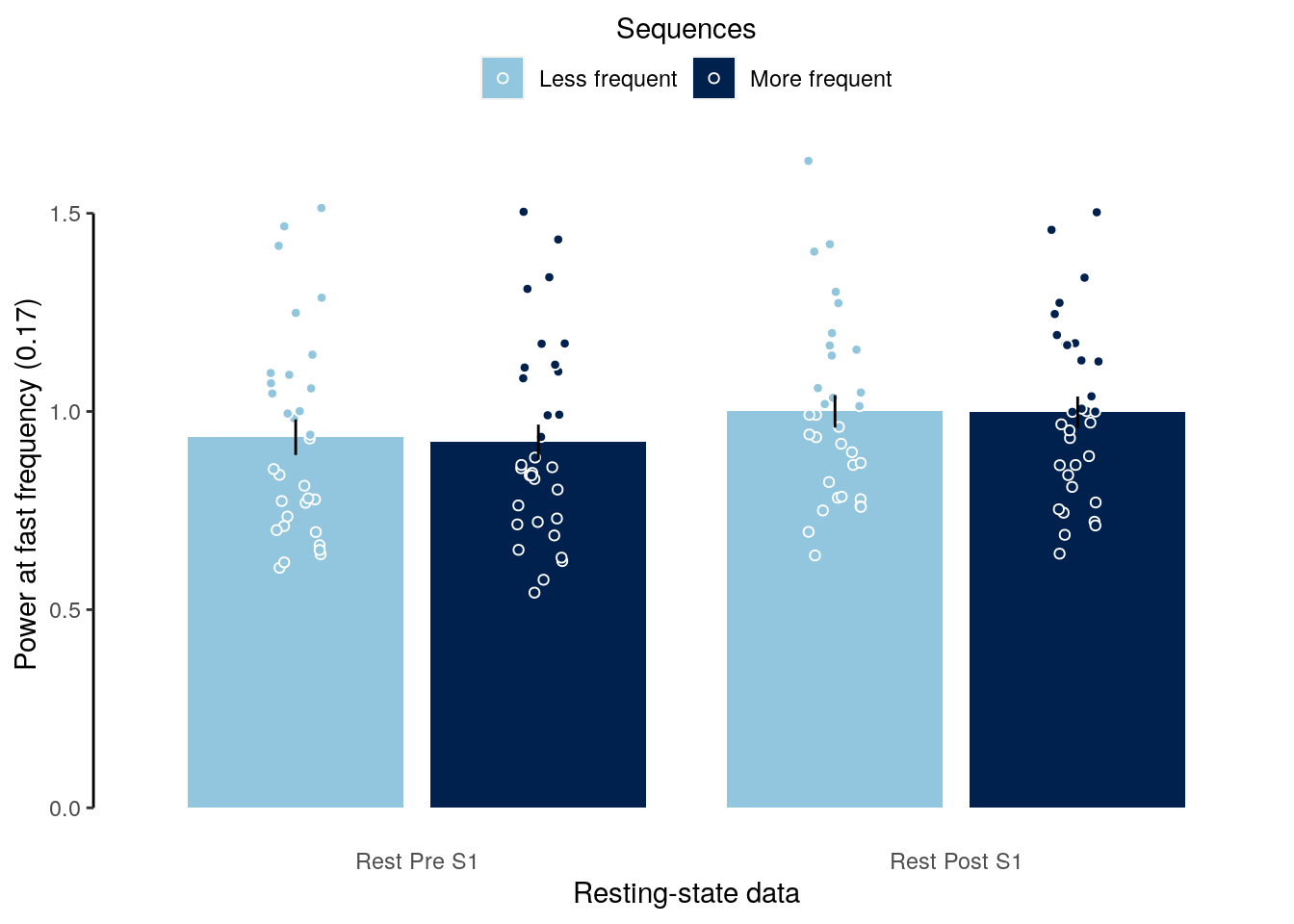
2.9.7.2 Source Data File Fig. 6c
dt_pred_rest_lsp_exp_seen %>%
filter(tITI %in% c("Rest Pre S1", "Rest Post S1")) %>%
filter(index == "power_index_fast") %>%
select(-classification, -index, -label, -num_seqs) %>%
write.csv(., file = file.path(path_sourcedata, "source_data_figure_6c.csv"),
row.names = FALSE)2.9.8 Figure 6
plot_grid(fig_freq_post, fig_freq_post_rel, fig_freq_exp_post, nrow = 1, ncol = 3,
labels = c("a", "b", "c"), rel_widths = c(3, 3, 3))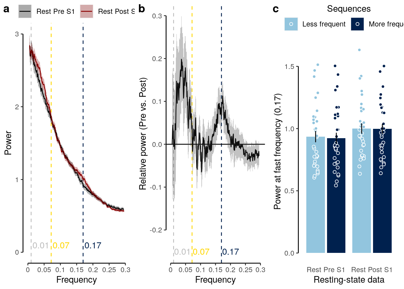
ggsave(filename = "highspeed_plot_decoding_resting_post.pdf",
plot = last_plot(), device = cairo_pdf, path = path_figures, scale = 1,
dpi = "retina", width = 9, height = 3)ggsave(filename = "wittkuhn_schuck_figure_6.pdf",
plot = last_plot(), device = cairo_pdf, path = path_figures, scale = 1,
dpi = "retina", width = 9, height = 3)2.9.9 Inserting sequence trials into rest
We create a function to sample sequence trials:
subseqsample = function(sequence, seq_size = 12, seq_num = 15) {
# initialize an empty array for the resulting indices:
index = rep(NA, length(sequence))
# calculate how much space would be allocated to gaps:
total_gaps = length(sequence) - seq_size * seq_num
# calculate random gaps
random_gaps = diff(sort(c(0, sample(1:(total_gaps + seq_num), seq_num), total_gaps + seq_num + 1)))
# we subtract 1 for each element of seq_num we added above:
random_gaps = random_gaps - 1
# make sure that the sum of random gaps matches the total gaps:
if (sum(random_gaps) != total_gaps) {warning("sum of gaps does not match!")}
# generate a random order of subsequences:
seq_order = sample(1:seq_num, seq_num)
# initialize the first starting point of potential sequences:
cstart = 0
# loop through all subsequences:
for (cseq in seq(1, seq_num)) {
# select the first random gap:
cgap = random_gaps[cseq]
# take the starting point and add the current random gap:
cstart = cstart + cgap + 1 # +1 because gap can be 0
# calculate the current subsequence index:
cidx = seq(cstart, (cstart + seq_size - 1))
# insert the random sequence index into the index array:
index[cidx] = seq_order[cseq]
# define a new starting position for the next subsequence:
cstart = max(cidx)
}
# return the indices:
return(index)
}
subseqsample(sequence = seq(1, 233))## [1] NA NA 14 14 14 14 14 14 14 14 14 14 14 14 NA NA 5 5 5 5 5 5 5 5 5
## [26] 5 5 5 NA NA NA 7 7 7 7 7 7 7 7 7 7 7 7 6 6 6 6 6 6 6
## [51] 6 6 6 6 6 8 8 8 8 8 8 8 8 8 8 8 8 NA NA 10 10 10 10 10 10
## [76] 10 10 10 10 10 10 4 4 4 4 4 4 4 4 4 4 4 4 NA NA NA NA NA 1 1
## [101] 1 1 1 1 1 1 1 1 1 1 3 3 3 3 3 3 3 3 3 3 3 3 NA 12 12
## [126] 12 12 12 12 12 12 12 12 12 12 NA NA NA 9 9 9 9 9 9 9 9 9 9 9 9
## [151] NA NA NA NA NA NA NA NA NA NA 11 11 11 11 11 11 11 11 11 11 11 11 NA NA NA
## [176] NA NA NA NA NA NA NA 2 2 2 2 2 2 2 2 2 2 2 2 NA NA NA NA NA NA
## [201] NA NA 15 15 15 15 15 15 15 15 15 15 15 15 NA NA NA NA 13 13 13 13 13 13 13
## [226] 13 13 13 13 13 NA NA NAWe randomly sample 15 sequences of 12 TRs each from resting state data and compare the mean frequency spectrum across those trials between resting state, fast and slow sequence trials.
dt_pred_rest_freq = dt_pred_conc_slope %>%
# we deselect post-task resting state data and assume on fixed ordering:
filter(!(tITI == "Rest Post S1") & sequence == 1) %>%
# filter for TRs in the forward and backward period only in sequence trials:
filter(!(tITI %in% c("32 ms", "2048 ms") & !(seq_tr %in% seq(2, 13)))) %>%
setDT(.) %>%
# select random chunks of TRs in the resting state data
.[tITI == "Rest Pre S1", by = .(classification, id), ":=" (trial_tITI = subseqsample(seq_tr))] %>%
# filter out all NA trials on resting state data
filter(!(is.na(trial_tITI) & tITI == "Rest Pre S1")) %>%
setDT(.) %>%
# assert that all the three conditions (two sequence trials and rest data) are present:
assert(in_set("32 ms", "2048 ms", "Rest Pre S1"), tITI) %>%
# calculate the frequency spectrum for every
.[, by = .(classification, id, tITI, trial_tITI), {
frequency_spectrum = stats::spectrum(
x = scale(slope), plot = FALSE, detrend = TRUE, demean = FALSE, spans = 5)
list(
num_trs = .N,
freq_bins = frequency_spectrum$freq,
spectrum = frequency_spectrum$spec
)}] %>% verify(all(num_trs %in% c(12, 6))) %>%
# normalize the frequencies per participant and trial to remove mean differences:
.[, by = .(classification, id, tITI, trial_tITI), ":=" (spectrum = spectrum/sum(spectrum))] %>%
# multiply the frequency levels by 1/TR:
transform(freq_bins = freq_bins * (1/1.25)) %>% setDT(.) %>%
# calculate the mean frequency spectrum per participant and condition:
.[, by = .(classification, id, tITI, freq_bins), .(
num_trials = .N,
mean_spec = mean(spectrum)
)] %>% verify(all(num_trials == 15)) %>%
# calculate the average frequency spectrum across all participants:
.[, by = .(classification, tITI, freq_bins), .(
num_subs = .N,
mean_spec = mean(mean_spec),
sem_upper = mean(mean_spec) + (sd(mean_spec)/sqrt(.N)),
sem_lower = mean(mean_spec) - (sd(mean_spec)/sqrt(.N))
)] %>%
verify(all(num_subs == 32))We insert a number of events with probabilities scaled at different SNR levels:
dt_pred_conc = dt_pred_all %>%
# we add a consecutive counter that will be used to concatenate data:
.[, by = .(classification, id, tITI, class), ":=" (t = seq(1, .N))] %>%
# we will focus all further analyses on the one-versus-rest classifier:
filter(classification == "ovr") %>% setDT(.)
# create separate dataframes for resting state data and sequence trial data:
dt_pred_rest_s1 = subset(dt_pred_conc, tITI == "rest_run-pre_ses-01")
dt_pred_seq_cut = subset(dt_pred_conc, tITI %in% c("32 ms", "2048 ms"))
speed_levels = unique(dt_pred_seq_cut$tITI)
num_speeds = length(speed_levels)
# define the number of SNR levels and sequence inserts:
snr_levels = c(4/5, 1/2, 1/4, 1/8, 0)
snr_levels_char = c("4/5", "1/2", "1/4", "1/8", "0")
num_snrs = length(snr_levels)
num_inserts = 6
insert_length = 12
# get the number of TRs during resting state and warn if incorrect:
num_rest_trs = max(dt_pred_rest_s1$t)
if (num_rest_trs != 233) {warning("number of resting state TRs incorrect")}
num_seq_trials = max(dt_pred_seq_cut$trial_tITI)
if (num_seq_trials != 15) {warning("number of sequence trials incorrect")}
num_subs = length(unique(dt_pred_rest_s1$id))
if (num_subs != 32) {warning("number of participants incorrect")}
# create a vector of seeds to make computations reproducible:
#seeds = seq(1, num_snrs * num_inserts * num_subs * num_speeds)
dt_pred_rest_insert <- list()
count = 1
for (sub in unique(dt_pred_rest_s1$id)) {
# sample random sequence trials to be cut out depending on the number of inserts:
cutout_trials = sort(sample(1:num_seq_trials, num_inserts, replace = FALSE))
# sample random insert sequences depending on the number of inserts (no overlap):
rest_seq = subseqsample(sequence = seq(1, num_rest_trs), seq_size = insert_length, seq_num = num_inserts * 2)
subsequence_starts = sort(sapply(X = seq(1, num_inserts * 2), FUN = function(x){which(rest_seq == x)[1]}))
insert_starts = sort(sample(subsequence_starts, num_inserts, replace = FALSE))
insert_stops = sort(insert_starts + insert_length - 1)
blend_starts = sort(setdiff(subsequence_starts, insert_starts))
blend_stops = sort(blend_starts + insert_length - 1)
for (ninserts in seq(1, num_inserts)) {
snr_index = 0
for (snr in snr_levels) {
snr_index = snr_index + 1
for (speed in speed_levels) {
# create a resting state data subset for the current settings:
dt_pred_rest_tmp = dt_pred_rest_s1 %>%
filter(id == sub) %>% setorder(classification, id, t, class) %>%
mutate(snr = snr) %>% mutate(insert = ninserts) %>% mutate(position_insert = position) %>%
mutate(speed = speed) %>% mutate(snr_char = snr_levels_char[snr_index]) %>%
mutate(prob_insert = probability) %>% mutate(prob_insert_blend = probability) %>%
mutate(insert_index = NA) %>% mutate(insert_start = NA) %>% setDT(.) %>%
verify(.[, by = .(classification, id, position), .(num_trs = .N)]$num_trs == num_rest_trs)
# loop through all events to cutout and insert fast sequences:
for (cevent in 1:ninserts) {
# create the sequence for sequence inserting:
insert_seq = seq(insert_starts[cevent], insert_stops[cevent])
# create the sequence for the blending rest trials:
blend_seq = seq(blend_starts[cevent], blend_stops[cevent])
# select the sequence from fast trials:
dt_pred_seq_cutout = dt_pred_seq_cut %>%
# filter for specififc participant and specific trial:
filter(id == sub & trial_tITI == cutout_trials[cevent]) %>%
# filter for specific speed and specific trs:
filter(tITI == speed & seq_tr %in% seq(2, insert_length + 1)) %>%
# sort by classification, id, timepoint and class (as rest data, see above):
setorder(classification, id, t, class) %>%
# multiply the probability with the current SNR level:
mutate(prob_snr = probability * snr)
# insert the snr-adjusted sequence trial probabilities:
dt_pred_rest_tmp$prob_insert[dt_pred_rest_tmp$t %in% insert_seq] = dt_pred_seq_cutout$prob_snr
# keep the position indices of the inserted sequence trials:
dt_pred_rest_tmp$position_insert[dt_pred_rest_tmp$t %in% insert_seq] = dt_pred_seq_cutout$position
# blend the snr-adjusted sequence trials with data from snr-adjusted res trials:
dt_pred_rest_tmp$prob_insert_blend[dt_pred_rest_tmp$t %in% insert_seq] = dt_pred_seq_cutout$prob_snr +
dt_pred_rest_tmp$probability[dt_pred_rest_tmp$t %in% blend_seq] * (1 - snr)
# create a new column with the (SNR-adjusted) sequence probabilities:
dt_pred_rest_tmp$prob_seq[dt_pred_rest_tmp$t %in% insert_seq] = dt_pred_seq_cutout$probability
dt_pred_rest_tmp$prob_seq_snr[dt_pred_rest_tmp$t %in% insert_seq] = dt_pred_seq_cutout$prob_snr
# include indices that indicate where data was inserted:
dt_pred_rest_tmp$insert_index[dt_pred_rest_tmp$t %in% insert_seq] = "inserted"
dt_pred_rest_tmp$insert_num[dt_pred_rest_tmp$t %in% insert_seq] = cevent
dt_pred_rest_tmp$insert_start[dt_pred_rest_tmp$t %in% min(insert_seq)] = 1
}
dt_pred_rest_insert[[count]] = dt_pred_rest_tmp
count = count + 1
}
}
}
}
# combine data in one datatable:
dt_pred_rest_insert <- do.call("rbind", dt_pred_rest_insert)
# calculate the differences in probability:
dt_pred_rest_insert$prob_diff = dt_pred_rest_insert$probability - dt_pred_rest_insert$prob_insert_blendPlot differences between inserted sequence speeds at different SNR levels:
cols_order = colorRampPalette(c('#4890F7', '#EB3C2D'), space = 'Lab')(5)
plot_data = subset(dt_pred_rest_insert, id == example_id) %>%
filter(insert_index == "inserted") %>% filter(speed == "32 ms") %>%
filter(insert == 1) %>%
transform(snr_char = factor(as.factor(snr_char), levels = c("4/5", "1/2", "1/4", "1/8", "0"))) %>% setDT(.)
fig_prob_diff_snr = ggplot(data = plot_data, aes(
x = as.factor(t), y = prob_seq_snr, color = snr_char, group = snr_char)) +
geom_line() + geom_point(alpha = 0.3) +
facet_wrap(~ class) + ylim(c(0,1)) +
scale_color_manual(values = cols_order, name = "SNR level") +
ylab("Probability (%)") + xlab("Time (TRs)") +
theme(strip.text = element_text(margin = margin(b = 2, t = 2, r = 2, l = 2))) +
coord_capped_cart(left = "both", bottom = "both", expand = TRUE) +
theme(legend.position = c(1, 0), legend.justification = c(1, 0)) +
scale_x_discrete(labels = label_fill(seq(1, 12, 1), mod = 11),
breaks = seq(min(plot_data$t), max(plot_data$t), 1)) +
theme(panel.border = element_blank(), axis.line = element_line()) +
theme(axis.line = element_line(colour = "black"),
panel.grid.major = element_blank(),
panel.grid.minor = element_blank(),
panel.border = element_blank(),
panel.background = element_blank())
fig_prob_diff_snr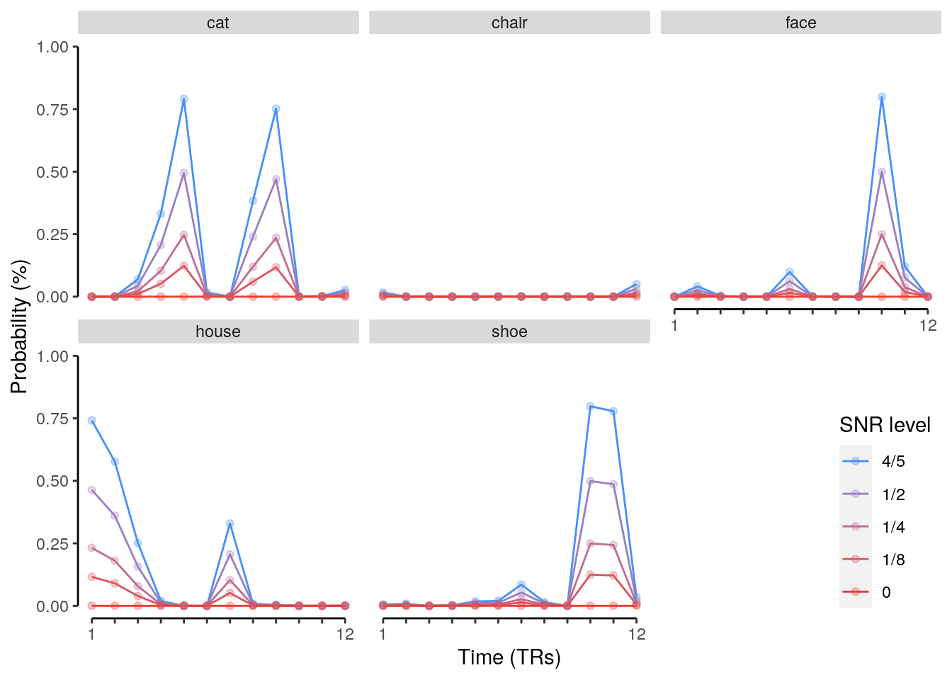
Plot differences in probability between true and augmented rest data.
plot_data = subset(dt_pred_rest_insert, id == example_id & speed == "32 ms") %>%
filter(snr_char %in% c("4/5", "1/4") & insert == c(2, 6)) %>%
mutate(snr_char = paste("SNR level:", snr_char)) %>%
mutate(insert = ifelse(insert == 1, paste(insert, "insert"), paste(insert, "inserts")))
# create data frame to plot rectangles where trials were inserted:
plot_rectangles = plot_data %>%
filter(insert_start == 1) %>%
mutate(xmin = t) %>%
mutate(xmax = ifelse(speed == "32 ms", xmin + 11, xmin + 11)) %>%
mutate(ymin = -100, ymax = 100)
fig_inserts = ggplot(data = plot_data, mapping = aes(
x = as.numeric(t), y = as.numeric(prob_diff * 100), group = as.factor(position))) +
geom_hline(aes(yintercept = 0), color = "gray") +
geom_line(mapping = aes(color = as.factor(position))) +
facet_grid(vars(as.factor(insert)), vars(fct_rev(as.factor(snr_char)))) +
geom_rect(data = plot_rectangles, aes(
xmin = xmin, xmax = xmax, ymin = ymin, ymax = ymax),
alpha = 0.2, inherit.aes = FALSE, show.legend = FALSE, fill = "gray") +
theme(legend.position = "top", legend.direction = "horizontal",
legend.justification = "center", legend.margin = margin(0, 0, 0, 0),
legend.box.margin = margin(t = 0, r = 0, b = -5, l = 0)) +
xlab("Time (TRs)") + ylab("Difference in probability (%)\nof sequence-free vs. -inserted rest") +
scale_colour_manual(name = "Serial position", values = color_events) +
coord_capped_cart(left = "both", bottom = "both", expand = TRUE,
xlim = c(0, 250), ylim = c(-100, 100)) +
guides(color = guide_legend(nrow = 1)) +
scale_x_continuous(labels = label_fill(seq(0, 250, 25), mod = 5),
breaks = seq(0, 250, 25)) +
theme(strip.text = element_text(margin = margin(b = 2, t = 2, r = 2, l = 2))) +
theme(panel.border = element_blank(), axis.line = element_line()) +
theme(axis.line = element_line(colour = "black"),
panel.grid.major = element_blank(),
panel.grid.minor = element_blank(),
panel.border = element_blank(),
panel.background = element_blank())
fig_inserts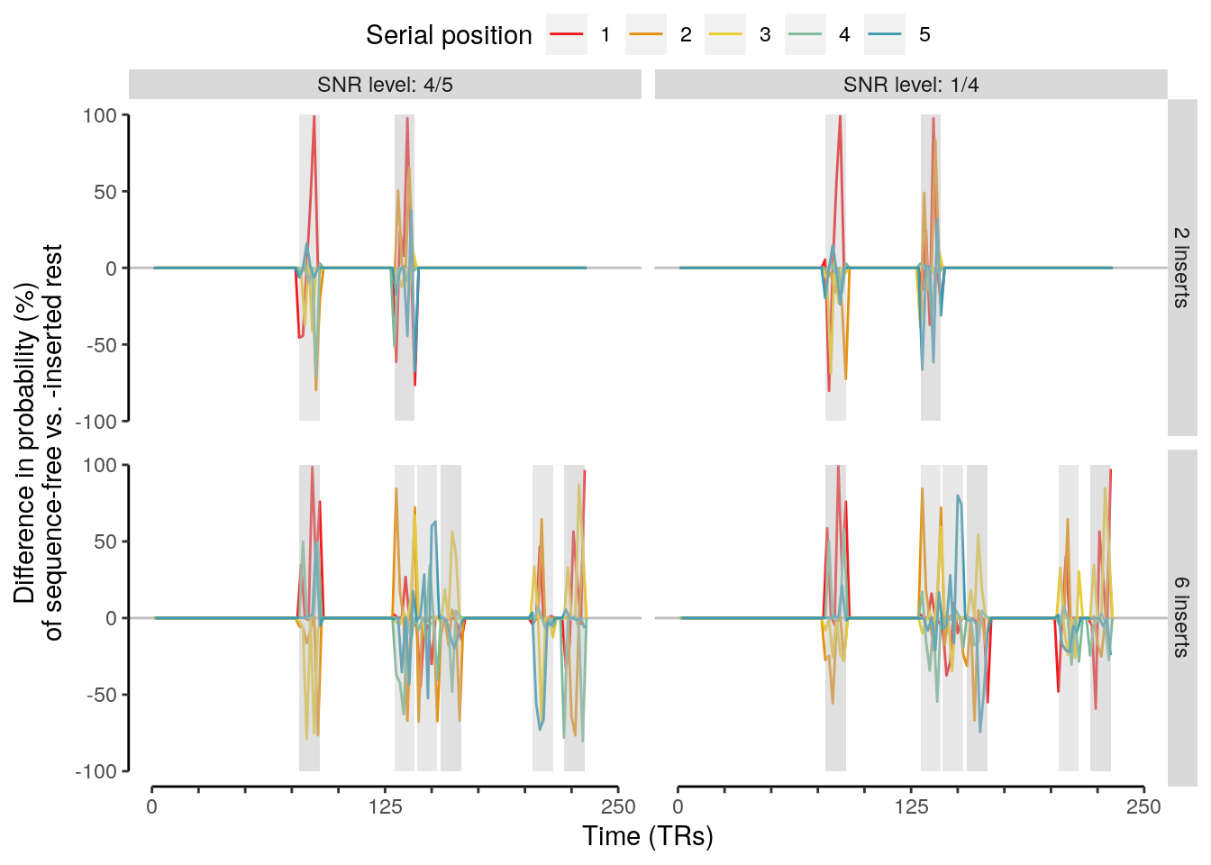
We calculate the slopes for each speed, snr and insert level.
Attention: This takes some time to run because a lot of linear models are estimated… About 13 minutes, OMG.
dt_pred_rest_insert %>%
verify(.[position != position_insert,]$insert_index == "inserted")## pred_label stim tr seq_tr stim_tr trial run_study session
## 1: other 1 1 NA 1 run-pre_ses-01 ses-01
## 2: other 1 1 NA 1 run-pre_ses-01 ses-01
## 3: other 1 1 NA 1 run-pre_ses-01 ses-01
## 4: house 1 1 NA 1 run-pre_ses-01 ses-01
## 5: other 1 1 NA 1 run-pre_ses-01 ses-01
## ---
## 2236796: other 233 233 NA 1 run-pre_ses-01 ses-01
## 2236797: other 233 233 NA 1 run-pre_ses-01 ses-01
## 2236798: other 233 233 NA 1 run-pre_ses-01 ses-01
## 2236799: other 233 233 NA 1 run-pre_ses-01 ses-01
## 2236800: other 233 233 NA 1 run-pre_ses-01 ses-01
## tITI id test_set classifier mask class
## 1: rest_run-pre_ses-01 sub-05 rest cat union cat
## 2: rest_run-pre_ses-01 sub-05 rest chair union chair
## 3: rest_run-pre_ses-01 sub-05 rest face union face
## 4: rest_run-pre_ses-01 sub-05 rest house union house
## 5: rest_run-pre_ses-01 sub-05 rest shoe union shoe
## ---
## 2236796: rest_run-pre_ses-01 sub-39 rest cat union cat
## 2236797: rest_run-pre_ses-01 sub-39 rest chair union chair
## 2236798: rest_run-pre_ses-01 sub-39 rest face union face
## 2236799: rest_run-pre_ses-01 sub-39 rest house union house
## 2236800: rest_run-pre_ses-01 sub-39 rest shoe union shoe
## probability classification condition trial_tITI probability_norm
## 1: 9.102896e-06 ovr rest 2 3.948250e-07
## 2: 2.443620e-02 ovr rest 2 6.931213e-04
## 3: 1.498180e-04 ovr rest 2 7.819401e-06
## 4: 9.465221e-01 ovr rest 2 3.597524e-02
## 5: 1.363089e-04 ovr rest 2 6.181498e-06
## ---
## 2236796: 7.106316e-07 ovr rest 2 3.988884e-08
## 2236797: 4.465901e-01 ovr rest 2 1.992650e-02
## 2236798: 1.003260e-03 ovr rest 2 4.685165e-05
## 2236799: 1.633766e-04 ovr rest 2 5.921457e-06
## 2236800: 4.423494e-02 ovr rest 2 1.814782e-03
## probability_zscore probability_cum position t snr insert
## 1: -0.4442724 3.948250e-07 5 1 0.8 1
## 2: -0.4585512 6.931213e-04 3 1 0.8 1
## 3: -0.4102144 7.819401e-06 4 1 0.8 1
## 4: 3.2804418 3.597524e-02 2 1 0.8 1
## 5: -0.4589078 6.181498e-06 1 1 0.8 1
## ---
## 2236796: -0.4322017 1.000000e+00 3 233 0.0 6
## 2236797: 1.6172451 1.000000e+00 4 233 0.0 6
## 2236798: -0.4657577 1.000000e+00 1 233 0.0 6
## 2236799: -0.4777543 1.000000e+00 5 233 0.0 6
## 2236800: -0.2521398 1.000000e+00 2 233 0.0 6
## position_insert speed snr_char prob_insert prob_insert_blend
## 1: 5 32 ms 4/5 9.102896e-06 9.102896e-06
## 2: 3 32 ms 4/5 2.443620e-02 2.443620e-02
## 3: 4 32 ms 4/5 1.498180e-04 1.498180e-04
## 4: 2 32 ms 4/5 9.465221e-01 9.465221e-01
## 5: 1 32 ms 4/5 1.363089e-04 1.363089e-04
## ---
## 2236796: 2 2048 ms 0 0.000000e+00 9.089871e-03
## 2236797: 4 2048 ms 0 0.000000e+00 2.291008e-04
## 2236798: 1 2048 ms 0 0.000000e+00 5.754922e-03
## 2236799: 5 2048 ms 0 0.000000e+00 4.862898e-05
## 2236800: 3 2048 ms 0 0.000000e+00 3.918135e-01
## insert_index insert_start prob_seq prob_seq_snr insert_num
## 1: <NA> NA NA NA NA
## 2: <NA> NA NA NA NA
## 3: <NA> NA NA NA NA
## 4: <NA> NA NA NA NA
## 5: <NA> NA NA NA NA
## ---
## 2236796: inserted NA 9.808940e-07 0 6
## 2236797: inserted NA 1.296404e-03 0 6
## 2236798: inserted NA 1.477866e-04 0 6
## 2236799: inserted NA 9.650072e-01 0 6
## 2236800: inserted NA 1.884389e-01 0 6
## prob_diff
## 1: 0.0000000000
## 2: 0.0000000000
## 3: 0.0000000000
## 4: 0.0000000000
## 5: 0.0000000000
## ---
## 2236796: -0.0090891599
## 2236797: 0.4463610056
## 2236798: -0.0047516613
## 2236799: 0.0001147476
## 2236800: -0.3475785457start_time = Sys.time()
# calculate the slope for each inserted and snr-adjusted rest data segment:
dt_pred_rest_insert_slope = dt_pred_rest_insert %>% setDT(.) %>%
# calculate the regression slopes for each id, trial, speed, snr, insert and TR:
.[, by = .(id, classification, speed, trial_tITI, insert, snr, snr_char, t, insert_num), .(
num_events = .N,
mean_position = mean(position),
mean_position_insert = mean(position_insert),
slope_rest = coef(lm(probability ~ position))[2] * (-1),
slope_insert = coef(lm(prob_insert_blend ~ position_insert))[2] * (-1),
sd_prob_rest = sd(probability),
sd_prob_insert = sd(prob_insert_blend)
# verify that the slope was calculated across five events with mean position of 3:
)] %>% verify(all(num_events == 5)) %>% verify(all(mean_position == 3)) %>%
verify(all(mean_position_insert == 3)) %>%
# sort the data table by speed, trial, number of inserts, snr level and time:
setorder(id, speed, trial_tITI, insert, snr, snr_char, t) %>%
# filter for one-versus-rest classification only:
filter(classification == "ovr") %>% setDT(.)
end_time = Sys.time()
print(end_time - start_time)## Time difference of 15.81017 minsPlot slopes with inserts:
colors = c(hcl.colors(5, "Cividis")[c(5,1)], "gray")
plot_rest = subset(dt_pred_rest_insert_slope, id == example_id) %>%
filter(snr_char %in% c("0", "4/5") & insert == c(6)) %>%
mutate(snr_char = paste("SNR level:", snr_char)) %>%
mutate(insert = ifelse(insert == 1, paste(insert, "insert"), paste(insert, "inserts")))
# create data frame to plot rectangles where trials were inserted:
plot_rectangles = plot_rest %>%
filter(!is.na(insert_num)) %>% setDT(.) %>%
.[, by = .(id, classification, speed, insert, snr, snr_char, insert_num), .(
xmin = min(t), xmax = max(t), ymin = -0.25, ymax = 0.25
)]
plot_inserts = plot_rest %>%
filter(!is.na(insert_num)) %>% setDT(.)
# plot the
fig_inserts_slopes = ggplot(data = plot_rest, mapping = aes(
x = as.numeric(t), y = as.numeric(slope_rest), color = fct_rev(speed))) +
geom_hline(aes(yintercept = 0), color = "black") +
geom_line(aes(color = "rest")) +
facet_grid(vars(as.factor(insert)), vars(as.factor(snr_char))) +
#facet_wrap(~ speed, nrow = 2, ncol = 1) +
facet_grid(vars(fct_rev(as.factor(speed))), vars(fct_rev(as.factor(snr_char)))) +
geom_rect(data = plot_rectangles, aes(
xmin = xmin, xmax = xmax, ymin = ymin, ymax = ymax, fill = speed),
alpha = 0.2, inherit.aes = FALSE, show.legend = FALSE) +
geom_line(data = plot_inserts, aes(
y = slope_insert, color = speed, group = interaction(insert_num, speed))) +
theme(legend.position = "top", legend.direction = "horizontal",
legend.justification = "center", legend.margin = margin(0, 0, 0, 0),
legend.box.margin = margin(t = 0, r = 0, b = -5, l = 0)) +
xlab("Time (TRs)") + ylab("Regression slope") +
scale_colour_manual(name = "Speed", values = colors) +
scale_fill_manual(name = "Speed", values = colors) +
coord_capped_cart(left = "both", bottom = "both", expand = TRUE, xlim = c(0, 250)) +
guides(color = guide_legend(nrow = 1)) +
scale_x_continuous(labels = label_fill(seq(0, 250, 25), mod = 5), breaks = seq(0, 250, 25)) +
theme(strip.text = element_text(margin = margin(b = 2, t = 2, r = 2, l = 2))) +
theme(axis.line = element_line(colour = "black"),
panel.grid.major = element_blank(),
panel.grid.minor = element_blank(),
panel.border = element_blank(),
panel.background = element_blank())
fig_inserts_slopes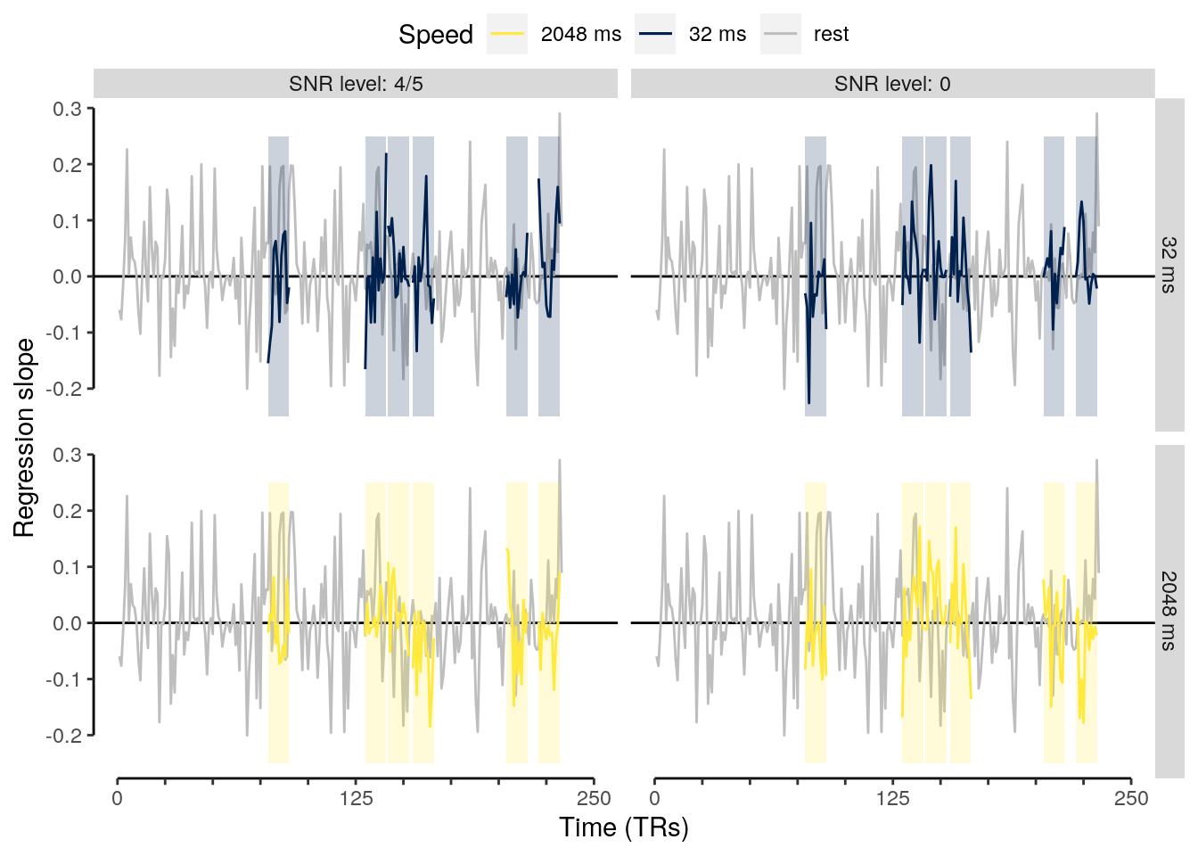
# select variable: either slopes or standard deviation:
insert_stat_func = function(dt, variable) {
dt_pred_rest_insert_slope_stat = dt %>%
# calculate mean slope coefficients across all augmented rest TRs:
.[, by = .(id, classification, speed, insert, snr, snr_char), .(
num_trs = .N,
mean_slope_rest = mean(abs(slope_rest)),
mean_slope_insert = mean(abs(slope_insert)),
mean_sd_prob_rest = mean(sd_prob_rest),
mean_sd_prob_insert = mean(sd_prob_insert)
)] %>% verify(all(num_trs == num_rest_trs)) %>%
# calculate the difference between the inserted and sequence-free rest data:
mutate(mean_slope_diff = mean_slope_insert - mean_slope_rest) %>%
mutate(mean_sd_diff = mean_sd_prob_insert - mean_sd_prob_rest) %>% setDT(.) %>%
# concuct a t-test comparing sequence-free vs. sequence-including rests:
.[, by = .(classification, speed, insert, snr, snr_char), {
ttest_results = t.test(get(variable), mu = 0, alternative = "two.sided")
list(
num_subs = .N,
mean_variable_diff = mean(get(variable)),
pvalue = ttest_results$p.value,
tvalue = round(ttest_results$statistic, 2),
df = ttest_results$parameter,
sem_upper = mean(get(variable)) + (sd(get(variable))/sqrt(.N)),
sem_lower = mean(get(variable)) - (sd(get(variable))/sqrt(.N))
)}] %>%
verify(all(num_subs == 32)) %>%
verify(all((num_subs - df) == 1)) %>%
# adjust p-values for multiple comparisons:
# check if the number of comparisons matches expectations:
.[, by = .(classification, speed), ":=" (
num_comp = .N,
pvalue_adjust = p.adjust(pvalue, method = "fdr", n = .N)
)] %>%
verify(all(num_comp == 30, na.rm = TRUE)) %>%
# round the original p-values according to the apa standard:
mutate(pvalue_round = round_pvalues(pvalue)) %>%
# round the adjusted p-value:
mutate(pvalue_adjust_round = round_pvalues(pvalue_adjust)) %>%
# create new variable indicating significance below 0.05
mutate(significance = ifelse(pvalue_adjust < 0.05, "*", "")) %>%
# log-transform the p-values:
mutate(pvalue_log = log(pvalue_adjust, base = 20)) %>%
# adjust the ordering of the snr levels:
transform(snr_char = factor(snr_char, levels = c("0", "1/8", "1/4", "1/2", "4/5"))) %>%
# set order:
setorder(classification, speed, insert, snr) %>% setDT(.)
return(dt_pred_rest_insert_slope_stat)
}
snr_insert_stat_slope = insert_stat_func(dt = dt_pred_rest_insert_slope, variable = "mean_slope_diff")
snr_insert_stat_sd = insert_stat_func(dt = dt_pred_rest_insert_slope, variable = "mean_sd_diff")
snr_insert_stat_slope %>% filter(pvalue_adjust < 0.05)## classification speed insert snr snr_char num_subs mean_variable_diff
## 1: ovr 2048 ms 1 0.250 1/4 32 -0.0006783505
## 2: ovr 2048 ms 1 0.500 1/2 32 -0.0005850498
## 3: ovr 2048 ms 2 0.125 1/8 32 -0.0012887714
## 4: ovr 2048 ms 2 0.250 1/4 32 -0.0015316188
## 5: ovr 2048 ms 2 0.500 1/2 32 -0.0015767316
## 6: ovr 2048 ms 3 0.125 1/8 32 -0.0015243604
## 7: ovr 2048 ms 3 0.250 1/4 32 -0.0019845733
## 8: ovr 2048 ms 3 0.500 1/2 32 -0.0022700075
## 9: ovr 2048 ms 4 0.125 1/8 32 -0.0018234399
## 10: ovr 2048 ms 4 0.250 1/4 32 -0.0025182348
## 11: ovr 2048 ms 4 0.500 1/2 32 -0.0030412334
## 12: ovr 2048 ms 4 0.800 4/5 32 -0.0017798178
## 13: ovr 2048 ms 5 0.125 1/8 32 -0.0023494214
## 14: ovr 2048 ms 5 0.250 1/4 32 -0.0032929623
## 15: ovr 2048 ms 5 0.500 1/2 32 -0.0041300272
## 16: ovr 2048 ms 5 0.800 4/5 32 -0.0026710542
## 17: ovr 2048 ms 6 0.125 1/8 32 -0.0028749268
## 18: ovr 2048 ms 6 0.250 1/4 32 -0.0040228464
## 19: ovr 2048 ms 6 0.500 1/2 32 -0.0050540671
## 20: ovr 2048 ms 6 0.800 4/5 32 -0.0033655876
## 21: ovr 32 ms 1 0.500 1/2 32 -0.0007120565
## 22: ovr 32 ms 1 0.800 4/5 32 -0.0006295727
## 23: ovr 32 ms 2 0.250 1/4 32 -0.0010584563
## 24: ovr 32 ms 2 0.500 1/2 32 -0.0015186540
## 25: ovr 32 ms 2 0.800 4/5 32 -0.0010774877
## 26: ovr 32 ms 3 0.250 1/4 32 -0.0015133809
## 27: ovr 32 ms 3 0.500 1/2 32 -0.0023493493
## 28: ovr 32 ms 3 0.800 4/5 32 -0.0017277111
## 29: ovr 32 ms 4 0.250 1/4 32 -0.0021098618
## 30: ovr 32 ms 4 0.500 1/2 32 -0.0032714726
## 31: ovr 32 ms 4 0.800 4/5 32 -0.0024898273
## 32: ovr 32 ms 5 0.125 1/8 32 -0.0016698843
## 33: ovr 32 ms 5 0.250 1/4 32 -0.0030286574
## 34: ovr 32 ms 5 0.500 1/2 32 -0.0045963901
## 35: ovr 32 ms 5 0.800 4/5 32 -0.0037752136
## 36: ovr 32 ms 6 0.125 1/8 32 -0.0021160060
## 37: ovr 32 ms 6 0.250 1/4 32 -0.0037482496
## 38: ovr 32 ms 6 0.500 1/2 32 -0.0056558378
## 39: ovr 32 ms 6 0.800 4/5 32 -0.0047157062
## classification speed insert snr snr_char num_subs mean_variable_diff
## pvalue tvalue df sem_upper sem_lower num_comp pvalue_adjust
## 1: 1.478176e-02 -2.58 31 -0.0004155991 -0.0009411019 30 2.463626e-02
## 2: 2.292923e-02 -2.39 31 -0.0003406151 -0.0008294845 30 3.439385e-02
## 3: 7.930664e-03 -2.84 31 -0.0008347125 -0.0017428303 30 1.486999e-02
## 4: 1.702289e-03 -3.44 31 -0.0010858070 -0.0019774306 30 3.928359e-03
## 5: 1.104530e-03 -3.60 31 -0.0011383525 -0.0020151108 30 2.975730e-03
## 6: 3.320638e-03 -3.18 31 -0.0010452262 -0.0020034945 30 6.641276e-03
## 7: 2.107488e-04 -4.20 31 -0.0015117028 -0.0024574437 30 7.903081e-04
## 8: 7.514246e-05 -4.56 31 -0.0017723750 -0.0027676400 30 3.757123e-04
## 9: 9.618887e-03 -2.76 31 -0.0011627596 -0.0024841202 30 1.697451e-02
## 10: 4.244833e-04 -3.95 31 -0.0018800452 -0.0031564244 30 1.414944e-03
## 11: 4.352357e-05 -4.75 31 -0.0024014025 -0.0036810644 30 2.611414e-04
## 12: 2.228288e-02 -2.41 31 -0.0010400625 -0.0025195732 30 3.439385e-02
## 13: 6.690586e-04 -3.78 31 -0.0017280208 -0.0029708220 30 2.007176e-03
## 14: 1.003238e-05 -5.27 31 -0.0026675704 -0.0039183541 30 7.524285e-05
## 15: 1.482092e-06 -5.93 31 -0.0034339971 -0.0048260574 30 1.482092e-05
## 16: 3.183047e-03 -3.20 31 -0.0018357737 -0.0035063347 30 6.641276e-03
## 17: 1.843268e-04 -4.24 31 -0.0021976012 -0.0035522523 30 7.899718e-04
## 18: 1.353303e-06 -5.97 31 -0.0033485066 -0.0046971863 30 1.482092e-05
## 19: 1.700336e-07 -6.70 31 -0.0042998034 -0.0058083308 30 5.101009e-06
## 20: 1.190292e-03 -3.57 31 -0.0024225906 -0.0043085846 30 2.975730e-03
## 21: 1.432149e-02 -2.60 31 -0.0004376641 -0.0009864490 30 2.864298e-02
## 22: 2.436143e-02 -2.37 31 -0.0003635874 -0.0008955580 30 4.299076e-02
## 23: 2.852956e-02 -2.30 31 -0.0005976709 -0.0015192416 30 4.693891e-02
## 24: 1.918252e-03 -3.39 31 -0.0010707586 -0.0019665494 30 5.231596e-03
## 25: 1.792355e-02 -2.50 31 -0.0006464789 -0.0015084965 30 3.360666e-02
## 26: 1.025117e-02 -2.73 31 -0.0009598135 -0.0020669484 30 2.365655e-02
## 27: 1.229776e-04 -4.39 31 -0.0018139422 -0.0028847564 30 5.270468e-04
## 28: 1.243207e-03 -3.55 31 -0.0012414282 -0.0022139941 30 3.729620e-03
## 29: 2.160017e-03 -3.35 31 -0.0014792606 -0.0027404630 30 5.400044e-03
## 30: 1.122824e-05 -5.23 31 -0.0026454949 -0.0038974502 30 8.421178e-05
## 31: 2.282997e-04 -4.17 31 -0.0018925106 -0.0030871439 30 7.880881e-04
## 32: 2.972798e-02 -2.28 31 -0.0009370586 -0.0024027101 30 4.693891e-02
## 33: 2.364264e-04 -4.16 31 -0.0022998922 -0.0037574227 30 7.880881e-04
## 34: 1.224176e-06 -6.00 31 -0.0038304320 -0.0053623483 30 1.836264e-05
## 35: 2.204612e-05 -4.99 31 -0.0030187922 -0.0045316350 30 1.322767e-04
## 36: 1.382206e-02 -2.61 31 -0.0013052532 -0.0029267589 30 2.864298e-02
## 37: 3.885401e-05 -4.79 31 -0.0029662079 -0.0045302913 30 1.942701e-04
## 38: 8.904749e-08 -6.93 31 -0.0048400824 -0.0064715932 30 2.671425e-06
## 39: 5.570983e-06 -5.47 31 -0.0038536909 -0.0055777215 30 5.570983e-05
## pvalue tvalue df sem_upper sem_lower num_comp pvalue_adjust
## pvalue_round pvalue_adjust_round significance pvalue_log
## 1: p = .01 p = .02 * -1.236271
## 2: p = .02 p = .03 * -1.124893
## 3: p = .008 p = .01 * -1.404802
## 4: p = .002 p = .004 * -1.849142
## 5: p = .001 p = .003 * -1.941851
## 6: p = .003 p = .007 * -1.673865
## 7: p < .001 p < .001 * -2.384421
## 8: p < .001 p < .001 * -2.632641
## 9: p = .01 p = .02 * -1.360616
## 10: p < .001 p = .001 * -2.190004
## 11: p < .001 p < .001 * -2.754067
## 12: p = .02 p = .03 * -1.124893
## 13: p < .001 p = .002 * -2.073292
## 14: p < .001 p < .001 * -3.169439
## 15: p < .001 p < .001 * -3.711770
## 16: p = .003 p = .007 * -1.673865
## 17: p < .001 p < .001 * -2.384563
## 18: p < .001 p < .001 * -3.711770
## 19: p < .001 p < .001 * -4.067811
## 20: p = .001 p = .003 * -1.941851
## 21: p = .01 p = .03 * -1.185969
## 22: p = .02 p = .04 * -1.050418
## 23: p = .03 p = .05 * -1.021089
## 24: p = .002 p = .005 * -1.753507
## 25: p = .02 p = .03 * -1.132622
## 26: p = .01 p = .02 * -1.249816
## 27: p < .001 p < .001 * -2.519658
## 28: p = .001 p = .004 * -1.866472
## 29: p = .002 p = .005 * -1.742929
## 30: p < .001 p < .001 * -3.131847
## 31: p < .001 p < .001 * -2.385360
## 32: p = .03 p = .05 * -1.021089
## 33: p < .001 p < .001 * -2.385360
## 34: p < .001 p < .001 * -3.640243
## 35: p < .001 p < .001 * -2.981112
## 36: p = .01 p = .03 * -1.185969
## 37: p < .001 p < .001 * -2.852812
## 38: p < .001 p < .001 * -4.283727
## 39: p < .001 p < .001 * -3.269769
## pvalue_round pvalue_adjust_round significance pvalue_logsnr_insert_stat_sd %>% filter(pvalue_adjust < 0.05)## classification speed insert snr snr_char num_subs mean_variable_diff
## 1: ovr 2048 ms 1 0.125 1/8 32 -0.001588456
## 2: ovr 2048 ms 1 0.250 1/4 32 -0.002161338
## 3: ovr 2048 ms 1 0.500 1/2 32 -0.002258520
## 4: ovr 2048 ms 2 0.125 1/8 32 -0.003392104
## 5: ovr 2048 ms 2 0.250 1/4 32 -0.004782021
## 6: ovr 2048 ms 2 0.500 1/2 32 -0.005477527
## 7: ovr 2048 ms 2 0.800 4/5 32 -0.002757742
## 8: ovr 2048 ms 3 0.125 1/8 32 -0.004351740
## 9: ovr 2048 ms 3 0.250 1/4 32 -0.006663250
## 10: ovr 2048 ms 3 0.500 1/2 32 -0.008337364
## 11: ovr 2048 ms 3 0.800 4/5 32 -0.005147277
## 12: ovr 2048 ms 4 0.125 1/8 32 -0.005312833
## 13: ovr 2048 ms 4 0.250 1/4 32 -0.008638720
## 14: ovr 2048 ms 4 0.500 1/2 32 -0.011345572
## 15: ovr 2048 ms 4 0.800 4/5 32 -0.007497486
## 16: ovr 2048 ms 5 0.125 1/8 32 -0.006762108
## 17: ovr 2048 ms 5 0.250 1/4 32 -0.010915281
## 18: ovr 2048 ms 5 0.500 1/2 32 -0.014435764
## 19: ovr 2048 ms 5 0.800 4/5 32 -0.010009554
## 20: ovr 2048 ms 6 0.125 1/8 32 -0.008342938
## 21: ovr 2048 ms 6 0.250 1/4 32 -0.013434359
## 22: ovr 2048 ms 6 0.500 1/2 32 -0.017926167
## 23: ovr 2048 ms 6 0.800 4/5 32 -0.012992737
## 24: ovr 32 ms 1 0.125 1/8 32 -0.001693297
## 25: ovr 32 ms 1 0.250 1/4 32 -0.002389709
## 26: ovr 32 ms 1 0.500 1/2 32 -0.002896940
## 27: ovr 32 ms 1 0.800 4/5 32 -0.002068804
## 28: ovr 32 ms 2 0.125 1/8 32 -0.003393000
## 29: ovr 32 ms 2 0.250 1/4 32 -0.004841657
## 30: ovr 32 ms 2 0.500 1/2 32 -0.005886753
## 31: ovr 32 ms 2 0.800 4/5 32 -0.003974918
## 32: ovr 32 ms 3 0.125 1/8 32 -0.004377856
## 33: ovr 32 ms 3 0.250 1/4 32 -0.006749073
## 34: ovr 32 ms 3 0.500 1/2 32 -0.008711215
## 35: ovr 32 ms 3 0.800 4/5 32 -0.006138349
## 36: ovr 32 ms 4 0.125 1/8 32 -0.005385562
## 37: ovr 32 ms 4 0.250 1/4 32 -0.008867752
## 38: ovr 32 ms 4 0.500 1/2 32 -0.012150993
## 39: ovr 32 ms 4 0.800 4/5 32 -0.009346154
## 40: ovr 32 ms 5 0.125 1/8 32 -0.006948115
## 41: ovr 32 ms 5 0.250 1/4 32 -0.011398804
## 42: ovr 32 ms 5 0.500 1/2 32 -0.015812024
## 43: ovr 32 ms 5 0.800 4/5 32 -0.012707678
## 44: ovr 32 ms 6 0.125 1/8 32 -0.008484621
## 45: ovr 32 ms 6 0.250 1/4 32 -0.013894101
## 46: ovr 32 ms 6 0.500 1/2 32 -0.019429020
## 47: ovr 32 ms 6 0.800 4/5 32 -0.016059415
## classification speed insert snr snr_char num_subs mean_variable_diff
## pvalue tvalue df sem_upper sem_lower num_comp pvalue_adjust
## 1: 3.368521e-02 -2.22 31 -0.0008737121 -0.002303200 30 4.393723e-02
## 2: 3.367757e-03 -3.18 31 -0.0014808274 -0.002841848 30 4.811081e-03
## 3: 1.303357e-03 -3.54 31 -0.0016196782 -0.002897363 30 2.300043e-03
## 4: 1.686447e-03 -3.44 31 -0.0024057638 -0.004378444 30 2.810746e-03
## 5: 2.997079e-05 -4.88 31 -0.0038028331 -0.005761210 30 7.492698e-05
## 6: 8.392514e-06 -5.33 31 -0.0044493967 -0.006505657 30 2.797505e-05
## 7: 2.341071e-02 -2.38 31 -0.0016011629 -0.003914320 30 3.192370e-02
## 8: 2.496835e-03 -3.29 31 -0.0030293279 -0.005674153 30 3.768319e-03
## 9: 1.830319e-05 -5.06 31 -0.0053453091 -0.007981192 30 4.991779e-05
## 10: 1.327036e-06 -5.97 31 -0.0069414033 -0.009733325 30 6.635179e-06
## 11: 2.512213e-03 -3.29 31 -0.0035820032 -0.006712550 30 3.768319e-03
## 12: 1.248916e-03 -3.55 31 -0.0038167624 -0.006808904 30 2.300043e-03
## 13: 2.603467e-06 -5.74 31 -0.0071327418 -0.010144698 30 1.115771e-05
## 14: 1.261535e-07 -6.81 31 -0.0096790083 -0.013012135 30 7.569209e-07
## 15: 6.513457e-04 -3.79 31 -0.0055195870 -0.009475384 30 1.302691e-03
## 16: 5.672893e-05 -4.66 31 -0.0053111141 -0.008213102 30 1.309129e-04
## 17: 3.308146e-08 -7.29 31 -0.0094186463 -0.012411917 30 2.481110e-07
## 18: 3.382055e-09 -8.14 31 -0.0126631113 -0.016208416 30 3.382055e-08
## 19: 7.890923e-05 -4.54 31 -0.0078069469 -0.012212161 30 1.690912e-04
## 20: 1.102961e-05 -5.23 31 -0.0067484624 -0.009937413 30 3.308882e-05
## 21: 1.826481e-09 -8.38 31 -0.0118310589 -0.015037659 30 2.739721e-08
## 22: 1.093311e-10 -9.49 31 -0.0160378511 -0.019814484 30 3.279932e-09
## 23: 5.540153e-06 -5.47 31 -0.0106185485 -0.015366926 30 2.077557e-05
## 24: 2.638296e-02 -2.33 31 -0.0009671234 -0.002419472 30 3.297870e-02
## 25: 1.852613e-03 -3.40 31 -0.0016876300 -0.003091788 30 2.646591e-03
## 26: 1.890219e-04 -4.24 31 -0.0022129877 -0.003580893 30 3.335680e-04
## 27: 7.136124e-03 -2.88 31 -0.0013506742 -0.002786933 30 9.307988e-03
## 28: 1.588893e-03 -3.46 31 -0.0024127652 -0.004373235 30 2.383339e-03
## 29: 2.058852e-05 -5.01 31 -0.0038761749 -0.005807139 30 4.411826e-05
## 30: 1.659514e-06 -5.89 31 -0.0048879858 -0.006885520 30 4.705985e-06
## 31: 6.730291e-04 -3.78 31 -0.0029229878 -0.005026848 30 1.121715e-03
## 32: 2.410296e-03 -3.30 31 -0.0030529137 -0.005702799 30 3.286767e-03
## 33: 1.437163e-05 -5.14 31 -0.0054360574 -0.008062088 30 3.316529e-05
## 34: 3.072465e-07 -6.49 31 -0.0073688533 -0.010053576 30 1.152175e-06
## 35: 1.220726e-04 -4.39 31 -0.0047402761 -0.007536422 30 2.288861e-04
## 36: 1.147917e-03 -3.58 31 -0.0038822514 -0.006888873 30 1.812500e-03
## 37: 1.451253e-06 -5.94 31 -0.0073751333 -0.010360370 30 4.705985e-06
## 38: 6.148641e-09 -7.92 31 -0.0106162964 -0.013685689 30 4.611481e-08
## 39: 1.725528e-06 -5.88 31 -0.0077567640 -0.010935545 30 4.705985e-06
## 40: 4.508704e-05 -4.74 31 -0.0054825232 -0.008413707 30 9.017408e-05
## 41: 1.438553e-08 -7.60 31 -0.0098989704 -0.012898638 30 8.631316e-08
## 42: 1.637226e-10 -9.33 31 -0.0141171669 -0.017506881 30 2.455840e-09
## 43: 1.962336e-07 -6.65 31 -0.0107965702 -0.014618785 30 8.410011e-07
## 44: 9.078517e-06 -5.30 31 -0.0068838300 -0.010085413 30 2.269629e-05
## 45: 9.410556e-10 -8.64 31 -0.0122852192 -0.015502982 30 9.410556e-09
## 46: 1.187518e-11 -10.42 31 -0.0175645175 -0.021293523 30 3.562555e-10
## 47: 3.197629e-08 -7.31 31 -0.0138611988 -0.018257631 30 1.598815e-07
## pvalue tvalue df sem_upper sem_lower num_comp pvalue_adjust
## pvalue_round pvalue_adjust_round significance pvalue_log
## 1: p = .03 p = .04 * -1.043148
## 2: p = .003 p = .005 * -1.781479
## 3: p = .001 p = .002 * -2.027827
## 4: p = .002 p = .003 * -1.960891
## 5: p < .001 p < .001 * -3.170843
## 6: p < .001 p < .001 * -3.499711
## 7: p = .02 p = .03 * -1.149771
## 8: p = .002 p = .004 * -1.863026
## 9: p < .001 p < .001 * -3.306415
## 10: p < .001 p < .001 * -3.980037
## 11: p = .003 p = .004 * -1.863026
## 12: p = .001 p = .002 * -2.027827
## 13: p < .001 p < .001 * -3.806542
## 14: p < .001 p < .001 * -4.704695
## 15: p < .001 p = .001 * -2.217596
## 16: p < .001 p < .001 * -2.984572
## 17: p < .001 p < .001 * -5.077019
## 18: p < .001 p < .001 * -5.742234
## 19: p < .001 p < .001 * -2.899148
## 20: p < .001 p < .001 * -3.443671
## 21: p < .001 p < .001 * -5.812544
## 22: p < .001 p < .001 * -6.521091
## 23: p < .001 p < .001 * -3.599031
## 24: p = .03 p = .03 * -1.138918
## 25: p = .002 p = .003 * -1.980979
## 26: p < .001 p < .001 * -2.672356
## 27: p = .007 p = .009 * -1.561182
## 28: p = .002 p = .002 * -2.015952
## 29: p < .001 p < .001 * -3.347641
## 30: p < .001 p < .001 * -4.094717
## 31: p < .001 p = .001 * -2.267525
## 32: p = .002 p = .003 * -1.908666
## 33: p < .001 p < .001 * -3.442900
## 34: p < .001 p < .001 * -4.564446
## 35: p < .001 p < .001 * -2.798076
## 36: p = .001 p = .002 * -2.107347
## 37: p < .001 p < .001 * -4.094717
## 38: p < .001 p < .001 * -5.638732
## 39: p < .001 p < .001 * -4.094717
## 40: p < .001 p < .001 * -3.109012
## 41: p < .001 p < .001 * -5.429485
## 42: p < .001 p < .001 * -6.617680
## 43: p < .001 p < .001 * -4.669534
## 44: p < .001 p < .001 * -3.569514
## 45: p < .001 p < .001 * -6.169254
## 46: p < .001 p < .001 * -7.262122
## 47: p < .001 p < .001 * -5.223709
## pvalue_round pvalue_adjust_round significance pvalue_log2.9.9.1 Figure 5f / 5g
Plot average slope regression coefficients and p-values:
cols_order = rev(colorRampPalette(c('#4890F7', '#EB3C2D'), space = 'Lab')(5))
plot_snr_insert = function(dt, variable) {
if (variable == "pvalue_log") {
yrange = seq(-10, 0, 1)
ylabel = "p-value\n(base-20 log-transformed)"
yintercept = -1
mod = 2
dt$sem_upper = 10; dt$sem_lower = 10;
}
else if (variable == "mean_slope_diff") {
variable = "mean_variable_diff"
yrange = seq(-0.007, 0.003, 0.001)
mod = 2
ylabel = "Regression slope\n(relative to pre-task rest)"
yintercept = 0
}
else if (variable == "mean_sd_diff") {
variable = "mean_variable_diff"
yrange = seq(-0.03, 0.01, 0.01)
mod = 1
ylabel = "SD of probability\n(relative to pre-task rest)"
yintercept = 0
}
ggplot(data = dt, mapping = aes(
x = as.factor(insert), y = as.numeric(get(variable)), group = as.factor(snr_char),
color = as.factor(snr_char), fill = as.factor(snr_char))) +
facet_wrap(~ fct_rev(as.factor(speed))) +
geom_hline(aes(yintercept = yintercept), color = "black", linetype = "dashed") +
geom_ribbon(aes(ymin = sem_lower, ymax = sem_upper), alpha = 0.5, color = NA) +
geom_line() + geom_point(pch = 15) +
theme(legend.position = "top", legend.direction = "horizontal",
legend.justification = "center", legend.margin = margin(0, 0, 0, 0),
legend.box.margin = margin(t = 0, r = 0, b = -5, l = 0)) +
xlab("Number of inserted sequence trials") + ylab(ylabel) +
coord_capped_cart(left = "both", bottom = "both", expand = TRUE, ylim = c(min(yrange), max(yrange))) +
guides(color = guide_legend(nrow = 1)) +
scale_color_manual(values = cols_order, name = "SNR level") +
scale_fill_manual(values = cols_order, name = "SNR level") +
scale_y_continuous(labels = label_fill(yrange, mod = mod), breaks = yrange) +
theme(strip.text = element_text(margin = margin(b = 2, t = 2, r = 2, l = 2))) +
theme(axis.line = element_line(colour = "black"),
panel.grid.major = element_blank(),
panel.grid.minor = element_blank(),
panel.border = element_blank(),
panel.background = element_blank())
}
fig_snr_pmat_slope = plot_snr_insert(dt = snr_insert_stat_slope, variable = "pvalue_log")
fig_snr_data_slope = plot_snr_insert(dt = snr_insert_stat_slope, variable = "mean_slope_diff")
fig_snr_pmat_sd = plot_snr_insert(dt = snr_insert_stat_sd, variable = "pvalue_log")
fig_snr_data_sd = plot_snr_insert(dt = snr_insert_stat_sd, variable = "mean_sd_diff")
fig_snr_pmat_slope; fig_snr_data_slope; fig_snr_pmat_sd; fig_snr_data_sd;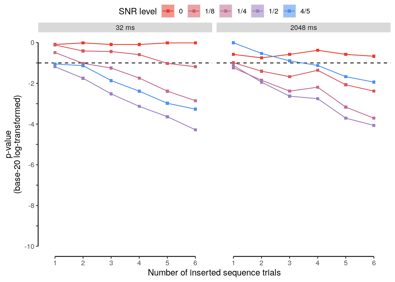
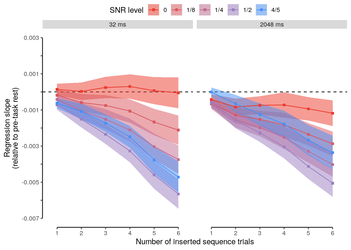
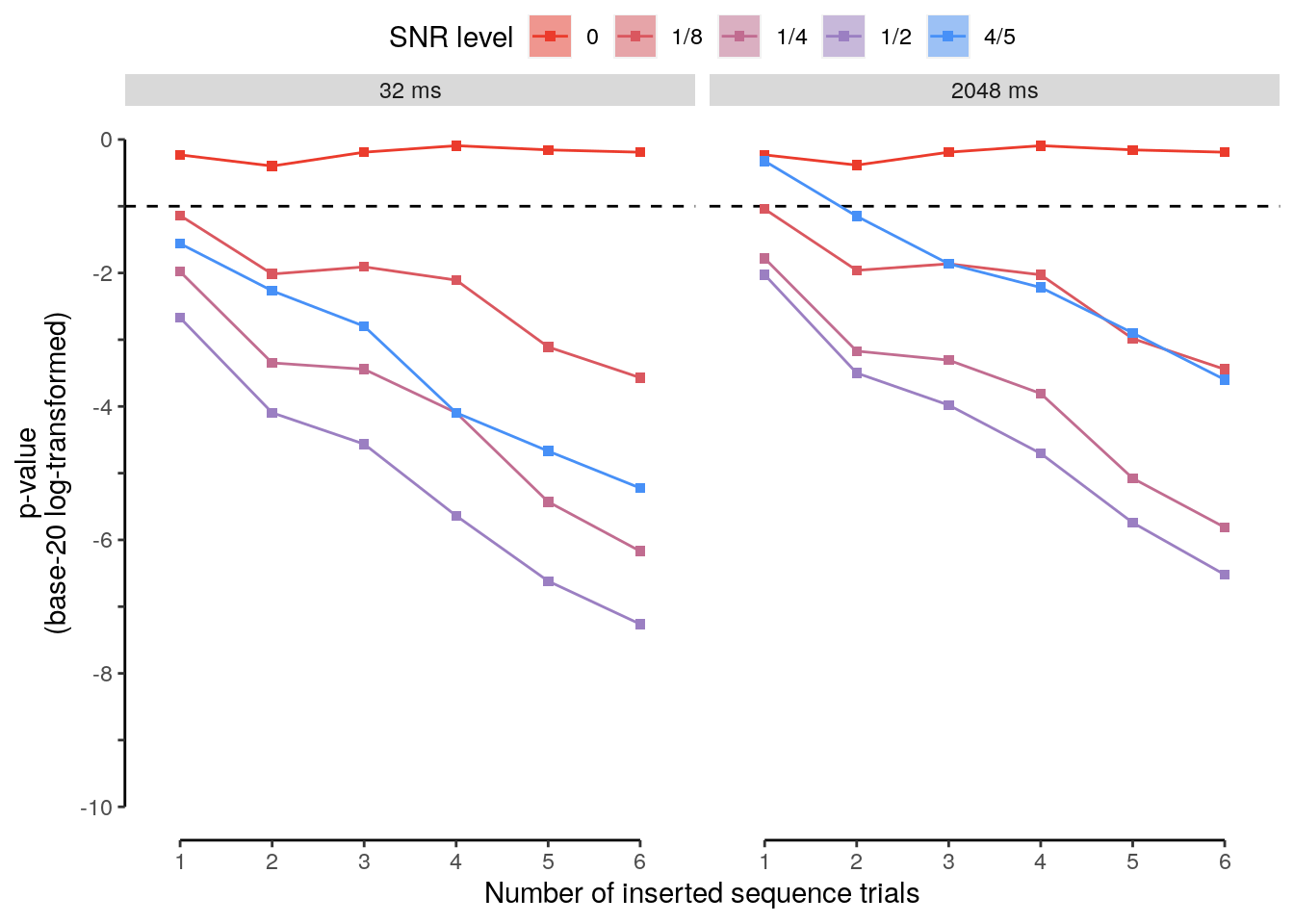
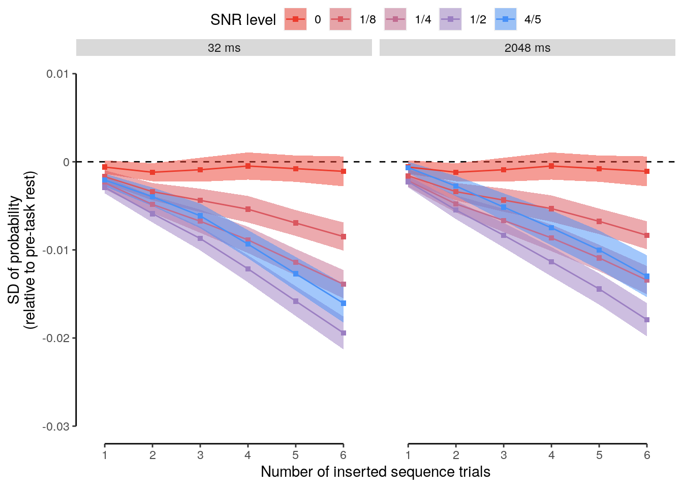
2.9.9.2 Source Data File Fig. 5f
snr_insert_stat_sd %>%
select(-num_subs, -classification, -pvalue, -tvalue, -df, -significance,
-num_comp, -pvalue_adjust, -pvalue_round, -pvalue_adjust_round) %>%
write.csv(., file = file.path(path_sourcedata, "source_data_figure_5f.csv"),
row.names = FALSE)2.9.9.3 Source Data File Fig. 5g
snr_insert_stat_sd %>%
select(-num_subs, -classification, -pvalue, -tvalue, -df, -significance,
-num_comp, -pvalue_adjust, -pvalue_round, -pvalue_adjust_round) %>%
write.csv(., file = file.path(path_sourcedata, "source_data_figure_5g.csv"),
row.names = FALSE)2.9.10 Frequency spectra (inserted)
2.9.10.1 Frequency spectra of augmented rest
We calculate the frequency spectra for sequence-free and sequence-inserted (fast and slow sequences) rest:
baseline = 1
# get frequency spectrum of fast and slow sequence data:
dt_pred_rest_insert_freq = dt_pred_rest_insert_slope %>%
# calculate the lomb scargle frequency spectra for every snr and insert level
.[, by = .(classification, id, speed, insert, snr, snr_char), {
frequency_spectrum = lsp(x = slope_insert, times = 1:.N, from = 0, to = 0.3, plot = FALSE, ofac = 2)
list(num_trs = .N, freq_bins = frequency_spectrum$scanned, power = frequency_spectrum$power,
filter_width = round(0.05/mean(diff(frequency_spectrum$scanned)))
)}] %>% verify(all(num_trs == 233)) %>% verify(length(unique(filter_width)) == 1) %>%
# smooth the frequency spectra:
.[, by = .(classification, id, speed, insert, snr, snr_char), ":=" (
power_smooth = stats::filter(power, rep(1/unique(filter_width), unique(filter_width))),
freq_bins_smooth = stats::filter(freq_bins, rep(1/unique(filter_width), unique(filter_width)))
)] %>%
# add a counter for the frequency spectrum
.[, by = .(classification, id, speed, snr, snr_char, insert), ":=" (bin = 1:.N)] %>%
# verify that the number of frequency bins is the same for all participants, snr, and insert levels:
verify(length(unique(.[, by = .(classification, id, speed, insert, snr), .(
num_bins = length(unique(bin)))]$num_bins)) == 1) %>%
# calculate power of every snr level relative to the snr 0 level:
.[, by = .(classification, id, speed, insert), ":=" (
power_smooth_rel = as.vector(sapply(X = sort(unique(snr)), FUN = function(x){
power_smooth[snr == x]/power_smooth[snr == 0]}) - baseline)
)]
# calculate the mean smoothed frequency for every snr and insert level across frequency bins:
dt_pred_rest_insert_freq_mean = dt_pred_rest_insert_freq %>%
.[, by = .(classification, speed, snr, snr_char, insert, freq_bins_smooth, bin), .(
num_subs = .N,
mean_power_smooth_rel = mean(power_smooth_rel),
sem_upper = mean(power_smooth_rel) + (sd(power_smooth_rel)/sqrt(.N)),
sem_lower = mean(power_smooth_rel) - (sd(power_smooth_rel)/sqrt(.N))
)] %>% verify(all(num_subs == 32))2.9.10.2 Figure 5h
colors_snr = rev(colorRampPalette(c('#4890F7', '#EB3C2D'), space = 'Lab')(5))
plot_data = dt_pred_rest_insert_freq_mean %>%
filter(!is.na(mean_power_smooth_rel)) %>%
filter(insert %in% c(2, 6)) %>%
mutate(insert = ifelse(insert == 1, paste(insert, "insert"), paste(insert, "inserts"))) %>%
# adjust the ordering of the snr levels:
transform(snr_char = factor(snr_char, levels = c("0", "1/8", "1/4", "1/2", "4/5"))) %>%
setDT(.)
freq_range = 0.01
num_plot_inserts = length(unique(plot_data$insert))
num_speed_inserts = length(unique(plot_data$speed))
frequency_expectation <- frequency_expectation[1:3,]
frequency_expectation_snr = frequency_expectation[1:3,] %>%
mutate(colors = c(hcl.colors(5, "Cividis")[c(1)], "gold", "gray")) %>%
.[rep(seq_len(nrow(.)), each = num_plot_inserts * num_speed_inserts), ] %>%
mutate(xmax = xintercept + freq_range, xmin = xintercept - freq_range) %>%
mutate(speed = rep(unique(plot_data$speed), num_plot_inserts * nrow(frequency_expectation))) %>%
mutate(insert = rep(rep(unique(plot_data$insert), each = 2), nrow(frequency_expectation))) %>%
transform(xintercept = ifelse(colors == "gray", 0.03, xintercept)) %>%
filter(colors != "gray")
fig_freq_lsp_insert = ggplot(data = plot_data, aes(
color = as.factor(snr_char), y = as.numeric(mean_power_smooth_rel), x = as.numeric(freq_bins_smooth))) +
geom_rect(data = frequency_expectation_snr, aes(
xmin = xmin, xmax = xmax, ymin = -0.2, ymax = 0.3),
alpha = 0.1, inherit.aes = FALSE, show.legend = FALSE, fill = frequency_expectation_snr$colors) +
#geom_vline(data = frequency_expectation_snr, aes(xintercept = xintercept),
# linetype = "dashed", color = frequency_expectation_snr$colors) +
geom_line() +
facet_grid(vars(insert), vars(fct_rev(as.factor(speed)))) +
geom_ribbon(aes(fill = snr_char, ymin = sem_lower, ymax = sem_upper),
alpha = 0.3, color = NA) +
#geom_text(data = frequency_expectation_snr, aes(
# x = xintercept + 0.03, y = -0.15, label = paste(round(xintercept, 2), "Hz")),
# color = frequency_expectation_snr$colors, size = 3) +
xlab("Frequency") + ylab("Power\n(relative to pre-task rest)") +
scale_color_manual(name = "SNR level", values = colors_snr, guide = FALSE) +
scale_fill_manual(name = "SNR level", values = colors_snr, guide = FALSE) +
theme(legend.position = "top", legend.direction = "horizontal",
legend.justification = "center", legend.margin = margin(0, 0, 0, 0),
legend.box.margin = margin(t = 0, r = 0, b = -5, l = 0)) +
coord_capped_cart(left = "both", bottom = "both", expand = TRUE,
xlim = c(0, 0.3), ylim = c(-0.2, 0.3)) +
#guides(color = guide_legend(nrow = 1)) +
theme(strip.text = element_text(margin = margin(b = 2, t = 2, r = 2, l = 2))) +
theme(axis.line = element_line(colour = "black"),
panel.grid.major = element_blank(),
panel.grid.minor = element_blank(),
panel.border = element_blank(),
panel.background = element_blank())
fig_freq_lsp_insert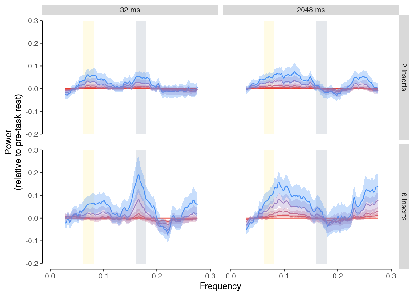
2.9.10.3 Source Data Fig. 5h
plot_data %>%
select(-classification, -bin, -num_subs) %>%
write.csv(., file = file.path(path_sourcedata, "source_data_figure_5h.csv"),
row.names = FALSE)2.9.10.4 Expected frequency ranges
dt_pred_rest_lsp_insert_exp = dt_pred_rest_insert_freq %>%
.[, by = .(classification, id, speed, snr, snr_char, insert), {
fast_min = which.min(abs(freq_bins_smooth - delta_freq_fast + freq_range))
fast_max = which.min(abs(freq_bins_smooth - delta_freq_fast - freq_range))
slow_min = which.min(abs(freq_bins_smooth - delta_freq_slow + freq_range))
slow_max = which.min(abs(freq_bins_smooth - delta_freq_slow - freq_range))
rest_min = which.min(abs(freq_bins_smooth - 0.03 + freq_range))
rest_max = which.min(abs(freq_bins_smooth - 0.03 - freq_range))
list(
fast_min = freq_bins_smooth[fast_min], fast_max = freq_bins_smooth[fast_max],
slow_min = freq_bins_smooth[slow_min], slow_max = freq_bins_smooth[slow_max],
power_index_fast = mean(power_smooth_rel[fast_min:fast_max]),
power_index_slow = mean(power_smooth_rel[slow_min:slow_max]),
power_index_rest = mean(power_smooth_rel[rest_min:rest_max])
)}] %>%
# melt all index variables into one column:
gather(grep("power", names(.), fixed = TRUE), key = "index", value = "power") %>% setDT(.) %>%
.[grepl("index_fast", index), label := paste0(round(delta_freq_fast, 2), "")] %>%
.[grepl("index_slow", index), label := paste0(round(delta_freq_slow, 2), "")] %>%
.[grepl("index_rest", index), label := paste0(round(delta_freq_rest, 2), "")] %>%
setorder(., classification, id, speed, snr, insert) %>%
# filter for specific inserts levels here:
filter(insert %in% c(2, 6)) %>% setDT(.)dt_pred_rest_lsp_insert_exp_mean = dt_pred_rest_lsp_insert_exp %>%
# filter out the irrelvant rest power index:
filter(index != "power_index_rest") %>% setDT(.) %>%
# compare the mean power in expected frequnecy for every SNR and insert level:
.[, by = .(classification, speed, insert, snr, snr_char, index), {
ttest_results = t.test(power, mu = 0, alternative = "two.sided", paired = FALSE)
list(
num_subs = .N,
pvalue = ttest_results$p.value,
tvalue = ttest_results$statistic,
df = ttest_results$parameter,
cohens_d = (mean(power) - 0)/sd(power)
)}] %>% verify(all(num_subs == 32)) %>% verify((num_subs - df) == 1) %>%
# adjust p-values for multiple comparisons:
# check if the number of comparisons matches expectations:
.[, by = .(classification, speed), ":=" (
num_comp = .N,
pvalue_adjust = p.adjust(pvalue, method = "fdr", n = .N)
)] %>%
# round the original p-values according to the apa standard:
mutate(pvalue_round = round_pvalues(pvalue)) %>%
# round the adjusted p-value:
mutate(pvalue_adjust_round = round_pvalues(pvalue_adjust)) %>%
# create new variable indicating significance below 0.05
mutate(significance = ifelse(pvalue_adjust < 0.05, "*", ""))
# filter for all p-values below the significance level:
dt_pred_rest_lsp_insert_exp_mean %>% filter(pvalue < 0.05)## classification speed insert snr snr_char index num_subs
## 1: ovr 2048 ms 2 0.125 1/8 power_index_slow 32
## 2: ovr 2048 ms 2 0.250 1/4 power_index_slow 32
## 3: ovr 2048 ms 2 0.500 1/2 power_index_slow 32
## 4: ovr 2048 ms 2 0.800 4/5 power_index_slow 32
## 5: ovr 2048 ms 6 0.800 4/5 power_index_slow 32
## 6: ovr 32 ms 2 0.800 4/5 power_index_fast 32
## 7: ovr 32 ms 2 0.800 4/5 power_index_slow 32
## 8: ovr 32 ms 6 0.800 4/5 power_index_fast 32
## pvalue tvalue df cohens_d num_comp pvalue_adjust pvalue_round
## 1: 0.037064838 2.178865 31 0.3851726 20 0.14825935 p = .04
## 2: 0.020549236 2.441117 31 0.4315327 20 0.10274618 p = .02
## 3: 0.008158507 2.826889 31 0.4997281 20 0.08158507 p = .008
## 4: 0.005626002 2.975570 31 0.5260115 20 0.08158507 p = .006
## 5: 0.014407380 2.592516 31 0.4582965 20 0.09604920 p = .01
## 6: 0.031706770 2.249760 31 0.3977051 20 0.26606660 p = .03
## 7: 0.039909990 2.144873 31 0.3791635 20 0.26606660 p = .04
## 8: 0.029710165 2.278960 31 0.4028671 20 0.26606660 p = .03
## pvalue_adjust_round significance
## 1: p = .15
## 2: p = .10
## 3: p = .08
## 4: p = .08
## 5: p = .10
## 6: p = .27
## 7: p = .27
## 8: p = .272.9.10.5 Figure 5i
cols_order = rev(colorRampPalette(c('#4890F7', '#EB3C2D'), space = 'Lab')(5))
plot_data = dt_pred_rest_lsp_insert_exp %>%
# add to inserts label:
mutate(insert = ifelse(insert == 1, paste(insert, "insert"), paste(insert, "inserts"))) %>%
# adjust the ordering of the snr levels:
transform(snr_char = factor(snr_char, levels = c("0", "1/4", "1/8", "1/2", "4/5"))) %>%
# filter out the irrelvant rest power index:
filter(index != "power_index_rest") %>% setDT(.)
fig_freq_exp_insert = ggplot(data = plot_data, aes(
y = power, x = fct_rev(label), fill = snr_char, color = snr_char, group = snr)) +
geom_bar(stat = "summary", fun = "mean", position = position_dodge(0.9),
width = 0.8) +
geom_point(position = position_jitterdodge(
jitter.width = 0.1, jitter.height = 0, seed = 2, dodge.width = 0.9),
alpha = 0.1, inherit.aes = TRUE, pch = 16) +
facet_grid(vars(insert), vars(fct_rev(as.factor(speed)))) +
stat_summary(fun.data = "mean_se", geom = "errorbar",
position = position_dodge(0.9), width = 0, color = "black") +
xlab("Predicted frequency") + ylab("Power\n(relative to pre-task rest)") +
coord_capped_cart(left = "both", bottom = "both", expand = TRUE, ylim = c(-0.1, 0.3)) +
scale_fill_manual(values = cols_order, name = "SNR level", guide = FALSE) +
scale_color_manual(values = cols_order, name = "SNR level", guide = FALSE) +
theme(axis.ticks.x = element_line(color = "white"), axis.line.x = element_line(color = "white")) +
theme(legend.position = "top", legend.direction = "horizontal",
legend.justification = "center", legend.margin = margin(t = 0, r = 0, b = 0, l = 0),
legend.box.margin = margin(t = 0, r = 0, b = 0, l = 0)) +
#guides(color = guide_legend(nrow = 1)) +
theme(strip.text = element_text(margin = margin(b = 2, t = 2, r = 2, l = 2))) +
theme(axis.line = element_line(colour = "black"),
panel.grid.major = element_blank(),
panel.grid.minor = element_blank(),
panel.border = element_blank(),
panel.background = element_blank())
fig_freq_exp_insert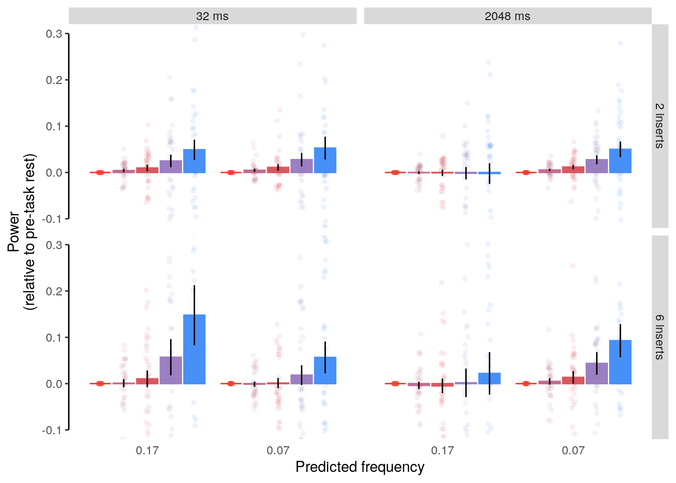
2.9.10.6 Source Data Fig. 5i
plot_data %>%
select(-classification, -fast_min, -fast_max, -slow_min, -slow_max) %>%
write.csv(., file = file.path(path_sourcedata, "source_data_figure_5i.csv"),
row.names = FALSE)2.9.11 Figure 5
panel_1 = plot_grid(fig_sd_prob, fig_mean_beta_abs, ncol = 2, labels = c("a", "b"))
panel_2 = plot_grid(fig_prob_slope, ncol = 1, labels = c("c"))
panel_3 = plot_grid(fig_freq_lsp, fig_freq_exp, ncol = 2, labels = c("d", "e"))
panel_4 = plot_grid(fig_snr_data_sd, fig_snr_pmat_sd, labels = c("f", "g"))
panel_5 = plot_grid(fig_freq_lsp_insert, fig_freq_exp_insert, labels = c("h", "i"))
plot_grid(plot_grid(panel_1, panel_2, ncol = 2), panel_3, panel_4, panel_5, ncol = 1)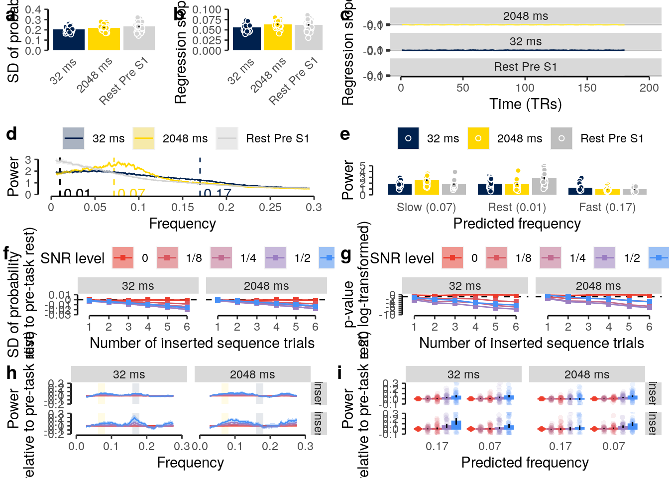
ggsave(filename = "highspeed_plot_decoding_rest.pdf",
plot = last_plot(), device = cairo_pdf, path = path_figures, scale = 1,
dpi = "retina", width = 10, height = 12)ggsave(filename = "wittkuhn_schuck_figure_5.pdf",
plot = last_plot(), device = cairo_pdf, path = path_figures, scale = 1,
dpi = "retina", width = 10, height = 12)2.10 Supplementary Figure
plot_grid(fig_prob_time_seq, fig_prob_diff_snr, fig_inserts, fig_inserts_slopes,
fig_snr_pmat_slope, fig_snr_data_slope, labels = "auto", ncol = 2, nrow = 3)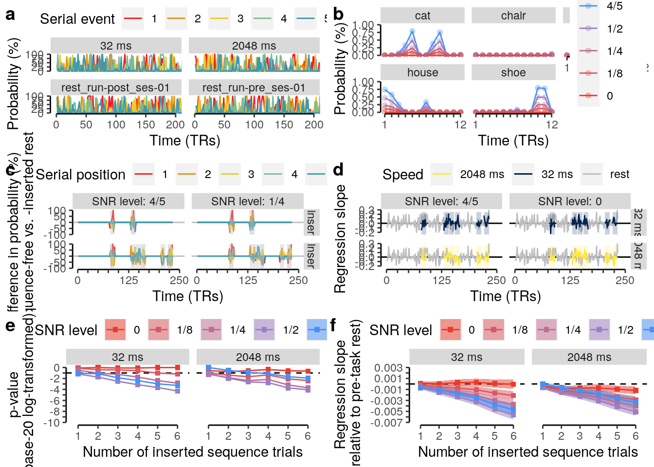
ggsave(filename = "highspeed_plot_decoding_rest_supplement.pdf",
plot = last_plot(), device = cairo_pdf, path = path_figures, scale = 1,
dpi = "retina", width = 10, height = 10)